Problem: Reduce the dimension of a data set, translating each data point into a representation that captures the “most important” features.
Solution: in Python
import numpy

def principalComponents(matrix):
    # Columns of matrix correspond to data points, rows to dimensions.

    deviationMatrix = (matrix.T - numpy.mean(matrix, axis=1)).T
    covarianceMatrix = numpy.cov(deviationMatrix)
    eigenvalues, principalComponents = numpy.linalg.eig(covarianceMatrix)

    # sort the principal components in decreasing order of corresponding eigenvalue
    indexList = numpy.argsort(-eigenvalues)
    eigenvalues = eigenvalues[indexList]
    principalComponents = principalComponents[:, indexList]

    return eigenvalues, principalComponents
Discussion: The problem of reducing the dimension of a dataset in a meaningful way shows up all over modern data analysis. Sophisticated techniques are used to select the most important dimensions, and even more sophisticated techniques are used to reason about what it means for a dimension to be “important.”
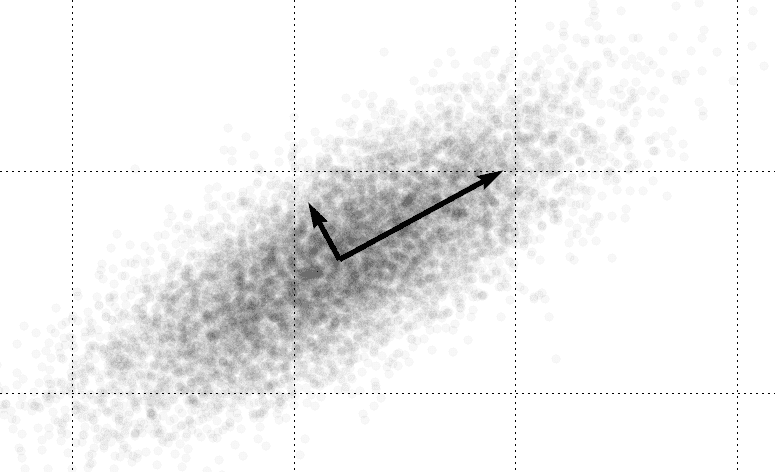
One way to solve this problem is to compute the principal components of a dataset*.* For the method of principal components, “important” is interpreted as the direction of largest variability. Note that these “directions” are vectors which may incorporate a portion of many or all of the “standard” dimensions in question. For instance, the picture below obviously has two different intrinsic dimensions from the standard axes.

The regular reader of this blog may recognize this idea from our post on eigenfaces. Indeed, eigenfaces are simply the principal components of a dataset of face images. We will briefly discuss how the algorithm works here, but leave the why to the post on eigenfaces. The crucial interpretation to make is that finding principal components amounts to a linear transformation of the data (that is, only such operations as rotation, translation, scaling, shear, etc. are allowed) which overlays the black arrows above on the standard axes. In the parlance of linear algebra, we’re re-plotting the data with respect to a convenient orthonormal basis of eigenvectors.
Here we first represent the dataset as a matrix whose columns are the data points, and whose rows represent the different dimensions. For example, if it were financial data then the columns might be the instances of time at which the data was collected, and the rows might represent the prices of the commodities recorded at those times. From here we compute two statistical properties of the dataset: the average datapoint, and the standard deviation of each data point. This is done on line 6 above, where the arithmetic operations are entrywise (a convenient feature of Python’s numpy library).
Next, we compute the covariance matrix for the data points. That is, interpreting each dimension as a random variable and the data points are observations of that random variable, we want to compute how the different dimensions are correlated. One way to estimate this from a sample is to compute the dot products of the deviation vectors and divide by the number of data points. For more details, see this Wikipedia entry.
Now (again, for reasons which we detail in our post on eigenfaces), the eigenvectors of this covariance matrix point in the directions of maximal variance, and the magnitude of the eigenvalues correspond to the magnitude of the variance. Even more, regarding the dimensions a random variables, the correlation between the axes of this new representation are zero! This is part of why this method is so powerful; it represents the data in terms of unrelated features. One downside to this is that the principal component features may have no tractable interpretation in terms of real-life phenomena.
Finally, one common thing to do is only use the first few principal components, where by ‘first’ we mean those whose corresponding eigenvalues are the largest. Then one projects the original data points onto the chosen principal components, thus controlling precisely the dimension the data is reduced to. One important question is: how does one decide how many principal components to use?
Because the principal components with larger eigenvalues correspond to features with more variability, one can compute the total variation accounted for with a given set of principal components. Here, the ‘total variation’ is the sum of the variance of each of the random variables (that is, the trace of the covariance matrix, i.e. the sum of its eigenvalues). Since the eigenvalues correspond to the variation in the chosen principal components, we can naturally compute the accounted variation as a proportion. Specifically, if $ \lambda_1, \dots \lambda_k$ are the eigenvalues of the chosen principal components, and $ \textup{tr}(A)$ is the trace of the covariance matrix, then the total variation covered by the chosen principal components is simply $ (\lambda_1 + \dots + \lambda_k)/\textup{tr}(A)$.
In many cases of high-dimensional data, one can encapsulate more than 90% of the total variation using a small fraction of the principal components. In our post on eigenfaces we used a relatively homogeneous dataset of images; our recognition algorithm performed quite well using only about 20 out of 36,000 principal components. Note that there were also some linear algebra tricks to compute only those principal components which had nonzero eigenvalues. In any case, it is clear that if the data is nice enough, principal component analysis is a vey powerful tool.
Want to respond? Send me an email, post a webmention, or find me elsewhere on the internet.