Last time we investigated the (very unintuitive) concept of a topological space as a set of “points” endowed with a description of which subsets are open. Now in order to actually arrive at a discussion of interesting and useful topological spaces, we need to be able to take simple topological spaces and build them up into more complex ones. This will take the form of subspaces and quotients, and through these we will make rigorous the notion of “gluing” and “building” spaces.
Subspaces of Euclidean Space
One of the simpler spaces we looked at last time was the circle “sitting inside” the real place $ \mathbb{R}^2$. But there is a disconnect in what makes this circle itself a topological space. Indeed, we can write down a description of the points in a circle, but what are the open sets?
The fact that the circle “sits inside” the real plane points us to the correct definition: we can take any open set in $ \mathbb{R}^2$ with the usual (Euclidean) topology, and define its intersection with the circle to be open. That is, the topology of the circle consists of all subsets of points of the circle which can be described this way. But there is nothing special about the circle here, so this makes for a good definition:
Definition: Let $ X$ be a topological space with topology $ T$ and $ Y \subset X$ a subset. The subspace topology of $ Y$ in $ X$ is defined as the topology
$$T’ = \left \{ Y \cap U : U \in T \textup{ is an open set of } X \right \}$$Let us verify that this is indeed a topology. Clearly the empty set and all of $ Y$ are in $ T’$ since $ \emptyset = \emptyset \cap Y, Y = Y \cap X$. Now given a collection of open sets $ Y \cap U_i$, their union is
$$\displaystyle \bigcup_i (Y \cap U_i) = Y \cap \left ( \bigcup_i U_i \right )$$And as the union $ \cup_i U_i$ is open in $ X$, the right hand side is in $ T’$. A similar argument shows that finite intersections are in $ T’$, so this is a valid topology.
Now there are two important spaces we need to define (as subspaces of Euclidean space) which will form the building blocks for all of our constructions. The first is the generalization of a sphere to any dimension.
Definition: The set of points $ S^1 = \left \{ (x,y) \in \mathbb{R}^2 : x^2 + y^2 = 1 \right \}$ is called the circle, or the 1-sphere, and is a topological space with the subspace topology of $ \mathbb{R}^2$.
Similarly, define $ S^n = \left \{ (x_1, \dots, x_{n+1}) \in \mathbb{R}^{n+1} : x_1^2 + \dots + x_{n+1}^2 = 1 \right \}$ to be the $ n$-sphere, a topological space when endowed with the subspace topology from $ \mathbb{R}^{n+1}$.
Finally, an $ n$-disk, denoted $ D^n$, is the set $ \left \{ (x_1, \dots , x_n) \in \mathbb{R}^n : x_1^2 + \dots + x_n^2 \leq 1 \right \}$. Note that for $ S^n$ the dimension of the ambient space is $ n+1$, but it is $ n$ for the disk.
The 0-sphere is hence a single point, the 2-sphere is the usual surface of a sphere in three dimensions, and we must resign to the futility of visualizing any of the higher dimensional spheres (for now, at least). We can think of the $ n$-disk as just the union of the $ n$-sphere and the open ball of radius 1 centered at the origin (a closed ball, perhaps?).
We can visualize the subspace topology on, for example, $ S^1$, as simply the unions of “open intervals” on the circle.

The second space we’d like to define is called the simplex (because it’s so “simple”).
Definition: The standard $ n$-simplex is the subset of $ \mathbb{R}^{n+1}$ taken as the convex hull of the $ n+1$ points:
$$(1,0,\dots,0), (0,1,0,\dots,0),\dots, (0,\dots,0,1)$$As taken with the subspace topology.

For example, the 0-simplex is a single point; the 1-simplex is a closed interval, which we usually write $ [0,1]$; the 2-simplex is a filled-in triangle; the 3-simplex is a filled-in tetrahedron, and so on.
The reader should note that topologically, the standard $ n$-simplex is equivalent to any convex hull of $ n+1$ points in general position. Indeed, it is not hard (but very tedious) to construct a homeomorphism between two such subsets. It is additionally obvious, but perhaps even harder to make rigorous, that an $ n$-simplex is homeomorphic to an $ n$-disk.
In fact, we will soon be able to define the sphere in terms of the n-simplex, and for our applications to programming, we will build all of our spaces purely from simplices. As such, we will call them “simplicial complexes.”
Now there is a very important distinction we have to make in defining topological spaces. Even though we view one space as “sitting inside” another, for the purpose of the topological space itself nothing else in the universe exists. The circle is a circle disregarding the ambient space it lives in or how it lives there. To make this rigorous, we call the act of viewing a space as “being inside” another space an embedding.
Definition: Let $ X, Y$ be arbitrary topological spaces. An embedding of $ X$ into $ Y$ is an injective map $ f:X \to Y$ which is a homeomorphism onto its image. That is, we need $ X$ to be homeomorphic to $ f(X)$, where the latter has the subspace topology of $ Y$.
Notice that the injectivity condition forces the image $ f(X)$ to not self-intersect. So last time our picture of the Klein Bottle was not an embedding in $ \mathbb{R}^3$. (Instead, it was an immersion, but we aren’t sophisticated enough to define this yet.)
Here are six examples of the circle $ S^1$ embedded into various topological spaces.

The first two we’ve already mentioned (the circle itself and the square, as viewed as subsets of the plane). The third (top right) is a more exotic embedding of $ S^1$ in the plane. The fourth (bottom left) is an embedding of the circle into three-dimensional Euclidean space. The fifth is an embedding of the circle as a subspace of the 2-sphere (realized as the equator). And the last is an example of a knot. In fact, topologically a knot is defined to be an embedding of $ S^1$ into $ \mathbb{R}^3$. The fascinating thing is that because we do not rely on the ambient space, the essential twists and tangles that make up a knot can be rich and varied. As long as the curve does not intersect itself, it is a valid embedding. There is much work devoted to classifying knots, but we will not go into it here.
Another important and simple example of an embedding is a simple path in a space. That is, an embedding of the 1-simplex $ [0,1]$ in $ X$. We can also have a plain old path, which is just a continuous (not necessarily injective) function $ [0,1] \to X$. These show up as the star of an important topological invariant, the fundamental group.
So we’re beginning to see precisely how wild and crazy these embeddings can be (and these examples are not even pathological!) which is part of what makes topology such a flexible and useful subject. Indeed, it’s going to get crazier once we start to glue spaces together.
Quotients of Sets: a Brief Tangent
In order to get a good feel for what a quotient space looks like, we need to be familiar with the idea of a quotient of sets. In our primer on set theory we pointed the reader to the Wikipedia page on equivalence relations, but since we’re actually going to use them in a nontrivial way, we should remind the reader of the basics. Roughly speaking, an equivalence relation is a generalization of “equality,” in that we define a new way to identify two elements of a set as “equalivalent.” The quotient of a set by an equivalence relation will then be the partition of the set into subsets of things which are identified as equivalent. Each subset in this partition is considered a single element of the quotient set. Let’s make this rigorous.
Definition: An equivalence relation $ \sim$ on a set $ X$ is a relation on $ X \times X$ which satisfies the following three properties:
- $ x \sim x$ for all $ x \in X$ (reflexivity).
- if $ x \sim y$ then $ y \sim x$ (symmetry).
- if $ x \sim y$ and $ y \sim z$ then $ x \sim z$ (transitivity).
These three properties are trivial properties of equality, and so they are reasonable constraints to enforce on a generalization of equality. For a nontrivial example of an equivalence relation (that is, one which is coarser than equality), consider the relation on the set of integers $ \mathbb{Z}$ where $ a \sim b$ if $ a$ and $ b$ have the same parity. It is easy to check this is an equivalence relation (we will have an even less trivial example in a minute).
Now every equivalence relation on a set $ X$ induces a natural partition of that set. The partitions correspond to equivalence classes of elements of $ x$ which are all equivalent to each other under $ \sim$. It is crucial to note that every partition gives rise to an equivalence relation as well (where two elements are equivalent if they are in the same piece of the partition). So we can define an equivalence relation by giving a partition, and vice versa.
What we’d like to do now is simply forget that elements of one equivalence class are different, and consider them collectively to be one element of a new set. This is the quotient.
Definition: Let $ X$ be a set and $ \sim$ an equivalence relation on $ X$. Define the quotient set of $ X$ by $ \sim$, denoted $ X / \sim$, to be the set of equivalence classes of $ \sim$.
A bit of notation: we will denote the equivalence class of an element $ x \in X$ using square brackets $ [x]$, and hence if any two elements $ x,y \in X$ are equivalent, we will write $ [x] = [y]$. This association defines an important map called the projection of $ X$ onto $ X/\sim$:
$$\pi : X \to X /\sim$$defined by $ \pi(x) = [x]$. Naturally, this map is a surjection (since every equivalence class is nonempty), and it actually has a very important universal property which we will only mention briefly here, but will explore in more depth in future posts. That is, if $ g: X \to Y$ is a function which preserves the equivalence relation structure (whenever $ x \sim y$, it must be that $ g(x) = g(y)$), then there is a unique map from the quotient $ f: X / \sim \to Y$ so that $ g$ “factors through” the quotient ($ g = f \circ \pi$). Since we somehow think of this projection as a “universal” construction, we sometimes call $ \pi$ the canonical projection. We are not saying much with that statement, but if it sounds mysterious the reader may ignore it. The important thing to take away from the projection map is that we will use it to define the open sets of $ X/\sim$ when we return to topological spaces.
A classic example of a quotient set is that of rational numbers. Indeed, when we think of two fractions, they are pairs of integers with a special equivalence relation. Specifically, $ a/b = c/d$ as numbers if and only if $ ad = bc$. To view this as a quotient set, let $ X$ be the set $ \mathbb{Z} \times (\mathbb{Z} – \left \{ 0 \right \})$ (that is, pairs of integers where the second is not zero). Define a relation $ \sim$ on $ X$ by $ (a,b) \sim (c,d)$ if $ ad – bc = 0$. It is easy to see this is an equivalence relation: reflexivity and symmetry are trivially satisfied. Suppose $ (a,b) \sim (c,d), (c,d) \sim (e,f)$. Then $ ad = bc, cf = ed,$ and since we want to prove $ af = be$ we can investigate the quantity $ af$:
$$(af)d = (ad)f = (bc)f = b(cf) = b(ed) = (be)d$$In particular, since $ d$ is a denominator (the second entry of a pair), it cannot be zero, and so we can divide through by $ d$ to get $ af = be$. There is a nice pictorial version of this argument as well, which we leave for the bored reader to think about.
So now that $ \sim$ is an equivalence relation, we can define the rational numbers $ \mathbb{Q}$ to be the quotient $ X/\sim$. As we just saw, this agrees with our usual notion of what it means for two fractions to be equal. Each equivalence class $ [(a,b)]$ in this set can be represented (arbitrarily) by the pair $ (a,b)$ which are relatively prime (since this uniquely determines a fraction). It is another story to ask whether the addition operation behaves well under this quotient (of course it does), and we will revisit this kind of question when we investigate the theory of groups.
Quotient Spaces
Now that we know what a quotient of a set is, it is not hard to define a quotient of a topological space. It is just the quotient as a set with a special topology.
Definition: Let $ X$ be a topological space and let $ \sim$ be an equivalence relation on $ X$, and let $ \pi : X \to X/\sim$ be the canonical projection map. The quotient topology on $ X/\sim$ is defined by declaring any subset $ U \in X/\sim$ to be open if its preimage $ \pi^{-1}(U)$ is open in $ X$.
This is a natural definition because we want to ensure that $ \pi$ is a continuous map of topological spaces, and every continuous map must satisfy this property. An explicit way to realize this is simply to take the union of all elements of the equivalence classes in $ U$, and check whether those elements are open as a subset of $ X$. We leave the formal verification that this satisfies the axioms of a topology to the reader.
Let’s turn to some examples. Let $ D$ be a disk in $ \mathbb{R}^2$ with the usual topology. Define a partition of $ D$ by putting every element of the boundary circle into one equivalence class, and putting every other element by itself. That is, our equivalence relation is $ x \sim y$ if $ x = y$ as points of $ X$, or if $ x,y$ are both on the boundary of the disk. Now the quotient space $ D/\sim$ “glues together” all points on the boundary of the disk (or rather, it contracts the boundary to a point). It is not hard to see that what we get is homeomorphic to the sphere $ S^2$. This animation should convince the reader.
An animation showing the process of glueing a disk along its boundary via a quotient (credit Wikipedia).
These kinds of visual arguments are extremely important to the topologist, because giving an explicit homeomorphism between this quotient space and the sphere would be quite rigorous, but an utter waste of time. The stubbornly interested reader would better spend his time investigating the Riemann Sphere, which epitomizes this homeomorphism.
Another important remark here is that even though our original disk could be embedded in $ \mathbb{R}^2$, the quotient space cannot be. As such, we should not be constrained by the ambient space of our original disk, and just imagine it (as in the animation above) floating in a sea of nothingness. Likewise with its quotient.
Likewise, we can take any topological space $ X$ and any subset $ U \in X$, and we can form the quotient of $ X$ by $ U$, denoted $ X/U$, by creating an analogous partition where all of $ U$ is in one subset of the partition, and every other point forms its own singleton class.
As a second example, let us take a filled in unit square in the plane, and observe various constructions of the spaces we introduced last time.

Note that this is homeomorphic to the disk, so we will just call it the disk. The first and simplest example is forming the Torus as a quotient of the disk by gluing opposite edges as shown.
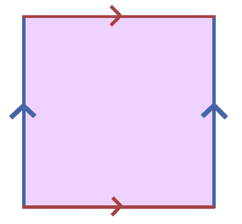
That is, we create a partition by identifying points on the boundary which are either horizontally opposite or vertically opposite (we only glue blue to blue and red to red). One can think of simply attaching one edge to the other in the direction of the arrows. The colors indicate which edges are glued to each other. Gluing one edge first gives a cylinder, and gluing the other edges together (which are now circles) gives the torus.
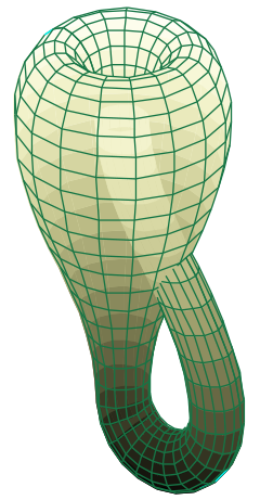
The second example is slightly more complicated: instead of gluing both of the edges in the same direction, switch one of the edges so that its glued in opposite directions. That is, glue according to the following picture:

Now imagine this as taking the cylinder again (gluing the edges which are still in the same direction) and gluing the boundary circles together, except with a twist. If this is hard to envision in three dimensions, that’s because it’s impossible. This space is the same Klein bottle we saw last time, and if you imagine one end of the cylinder passing through the cylinder meet the other boundary circle from inside, you start to see this picture:
The neat thing about this is that we can still define the quotient and it will make sense regardless of whether we can picture it. Part of the allure of topological spaces is that we can define them so simply, but understanding their structure is so difficult.
A perfect example of this, and our last space to be defined as a quotient of a disk, is the real projective plane $ \mathbb{R}\textup{P}^2$. In particular, it’s the quotient of the disk where both sides are glued in opposite directions.

Perhaps it is easier to see this as a quotient of a “circular” disk, since we are really just identifying the top and bottom semicircles by declaring antipodal points to be equivalent. Convince yourself that the following construction is homeomorphic to that in the above picture:

Now $ \mathbb{R}\textup{P}^2$ is the most mysterious of the spaces we’ve seen so far, but for mathematicians it is a standard object. Another way to realize it is as a quotient of $ \mathbb{R}^3 – \left \{ (0,0,0) \right \}$ by identifying two points to be the same if they lie on the same line through the origin.
We will explore the properties of $ \mathbb{R}\textup{P}^2$, the Klein bottle, and the torus in future topology primers, but for now we still need to work on building up spaces.
Disjoint Unions and Gluing along a Function
Perhaps more useful than gluing one space to itself is gluing one space to another.
Definition: Let $ X,Y$ be topological spaces and let $ f:U \to Y$ be a continuous function on some subspace $ U \subset X$. To glue $ X$ to $ Y$ along $ f$ is to form the quotient space $ (X \coprod Y)/\sim$, where $ \coprod$ denotes a disjoint union and $ \sim$ is defined by declaring the only non-trivial relations to be $ x \sim f(x)$. We denote this space $ X \coprod_f Y$.
The disjoint union is just a formality: it says that even if our two spaces $ X$ and $ Y$ come from the same ambient space (say, two copies of the unit disk in the plane), we consider the points from $ X$ to be formally disjoint from those of $ Y$, and then take a union. There is a rigorous way to view this, but we will not need it on this blog until we reach category theory.
For example, let’s glue two disks together along their boundary to form $ S^2$. That is, let $ X = Y = D^2$, and consider $ S^1 \subset D^2$ to be the boundary circle. Define $ f:S^1 \to Y$ by mapping isomorphically onto the boundary of $ Y$. Then the quotient $ X \coprod_f Y$ is a sphere. To visualize this concretely, just imagine taking two open hemispheres and gluing them along their common equator.

In a similar way, we can achieve the higher dimensional $ n$-sphere by gluing two $ n$-disks along their common boundary $ S^{n-1}$. That is, every higher dimensional sphere is comprised of two “hemispheres.” This gives us one potentially awkward way of viewing $ S^3$ by taking two filled in spheres ($ D^3$) and gluing them together along their boundary surfaces. Note that this would involve contorting one of the spheres into a very embarrassing position, and it is considered rude to do it in public.
Now that we’ve unlocked this new ability to glue spaces together, there is a myriad of interesting spaces we can build and tinker with. As gratifying and fruitful as this may be, we should have some way of organizing a class of such spaces so that we may prove theorems about all of them simultaneously. This will be the class of simplicial complexes.
Simplicial Complexes
Now we will construct a large class of topological spaces which are particularly tractable for analysis and manipulation in a computer. They are called simplicial complexes, and they are built up from the $ n$-simplices we defined earlier by gluing along sub-simplices.
Recall that an $ n$-simplex was the convex hull of any $ n+1$ points in general position in $ \mathbb{R}^{n+1}$. Let $ \sigma$ be an $ n$-simplex. We add a few natural definitions by calling each of the original $ n+1$ points used to define $ \sigma$ a vertex of $ \sigma$, and the convex hull of any subset of the vertices of $ \sigma$ a face of $ \sigma$. In particular, this means that for a $ 3$-simplex (a tetrahedron), we consider each triangle on the boundary, each edge connecting two vertices, and each vertex itself a “face” of the simplex. If we need to distinguish a certain kind of face, we will prefix it by the number of points used to define it. i.e., an edge of the tetrahedron would be a $ 2$-face.
Definition: A simplicial complex is a topological space realized as a union of any collection of simplices (of possibly varying dimension) $ \Sigma$ which has the following two properties:
- Any face of a simplex $ \Sigma$ is also in $ \Sigma$.
- The intersection of any two simplices of $ \Sigma$ is also a simplex of $ \Sigma$.
We can realize a simplicial complex by gluing together pieces of increasing dimension. First start by taking a collection of vertices (0-simplices) $ X_0$. Then take a collection of intervals (1-simplices) $ X_1$ and glue their endpoints onto the vertices in any way. Note that because we require every face of the intervals are again simplices in our complex, we must glue every endpoint of an interval onto one of the vertices in $ X_0$. Continue this process with $ X_2$, a set of 2-simplices, and so on until you reach a terminating set $ X_n$ (or not, but on this blog our complexes always will). It is easy to see that the union of the $ X_i$ form a simplicial complex. Define the dimension of the cell complex $ X = X_0 \cup \dots \cup X_n$ to be $ n$.
There are some picky restrictions on how we glue things that we should mention. For instance, we could not contract all edges of a 2-simplex $ \sigma$ and glue it all to a single vertex in $ X_0$. The reason for this is that $ \sigma$ would no longer be a 2-simplex! Indeed, we’ve destroyed its original vertex set, and it is no longer a convex hull. The gluing process hence needs to preserve the original simplex’s boundary. If we want to be more flexible with our gluing rules, we would need a more general structure called a CW-complex. For all intents and purposes, CW-complexes and simplicial complexes are equivalent, but CW-complexes are much more difficult to represent in a computer (this author does not believe they can be, because they allow for arbitrary kinds of quotients). We will not discuss them here.
Despite the restrictions, we can still build a wide variety of spaces as simplicial complexes. For instance, a disk is homeomorphic to any 2-simplex, and the circle can be realized as three 1-simplices glued to form a triangle’s boundary. Even better, we can realize the torus, the klein bottle, and the projective plane as simplicial complexes by decomposing the square into two triangles, and gluing the boundaries together as we did earlier in this post. In fact, most spaces we’ve considered thus far is a simplicial complex. The easiest example of a space which cannot be realized as a simplicial complex is an open ball. Since all of our $ n$-simplices are closed as subsets of $ \mathbb{R}^{n+1}$, and we are taking finite unions of them (fudging a few details), the result will always be a closed subset of $ \mathbb{R}^m$ for some $ m$.
We’ve had kind of a whirlwind ride through what should be a more slowly-digested subject. While there is still more theory to come before we can reach the applications, we’re about to depart from the world of point-set topology and move toward algebraic topology. That is, we’re going to construct topological invariants (recall, properties preserved by homeomorphisms) that are based in algebra. But point-set topology is still quite an interesting subject, and we’d like to point the reader to a few books for further reading. The largest and most mathematical is a textbook by Munkres. A denser but shorter paperback text (which this author learned the subject from originally) is by Gamelin and Greene. Perhaps the best text for a beginner would be that of Mendelson, as the other two go far beyond what is covered in that text.
In any event, next time we’ll start to develop these algebraic invariants, and to do that we have to develop some algebra. Until then!
Want to respond? Send me an email, post a webmention, or find me elsewhere on the internet.