Being part of the subject of algebraic topology, this post assumes the reader has read our previous primers on both topology and group theory. As a warning to the reader, it is more advanced than most of the math presented on this blog, and it is woefully incomplete. Nevertheless, the aim is to provide a high level picture of the field with a peek at the details.
An Intuitive Topological Invariant
Our eventual goal is to get comfortable with the notion of the “homology group” of a topological space. That is, to each topological space we will associate a group (really, a family of groups) in such a way that whenever two topological spaces are homeomorphic their associated groups will be isomorphic. In other words, we will be able to distinguish between two spaces by computing their associated groups (if even one of the groups is different).
In general, there may be many many ways to associate a group with an object (for instance, it could be a kind of symmetry group or a group action). But what we want to do, and what will motivate both this post and the post on homology, is figure out a reasonable way to count holes in a space. Of course, the difficult part of this is determining what it means mathematically to have a “hole” in a space.
The simplest example of this is a circle $ S^1$:

That is, we think of this space (not embedded in any particular Euclidean space) as having a single one-dimensional “hole” in it. Furthermore, a sphere $ S^2$ has a two-dimensional “hole” in it (the hollow interior).
So our approach to make “holes” rigorous will follow a commonly tread mathematical trail: come up with a definition which fits with our intuition for these special cases, and explore how the definition generalizes to other cases. In this post we will stick exclusively to one-dimensional holes (with a small exception when we take a peek at the chaos of higher homotopy groups at the end of this post), and the main object we use to represent them is called the fundamental group.
On the other hand, we will find that the fundamental group is too unwieldy to compute (and for deep reasons). Since we want to be able to readily compute the number of holes in twisted and tied-up spaces, we will need to scrap the fundamental group and try something else. Instead, we’ll derive various kinds of other groups associated to a topological space, which will collectively fall under the name homology groups. After that, we will be able to actually write a program which computes homology of sufficiently nice spaces (simplicial complexes). Our main use for this will actually be to compute the topological features of a data set, but let’s cross that bridge when we get to it.
For now, we will develop the idea of homotopy and the fundamental group. It will show us how to think geometrically about topology and give us our first interplay between topology and algebra.
Paths and Homotopy
For the remainder of this post (and all of our future posts in topology), a map will always mean a continuous function. The categorical way to say this, which we will use increasingly often as we approach more advanced topics, is by saying that continuous maps are “the morphisms in the category of topological spaces.”
So we define by a path in a topological space $ X$ to be a map $ f(t):[0,1] \to X$ (that is, a continuous function $ [0,1] \to X$). There are many kinds of paths in a space:

An example of three paths in the plane.
Paths are necessarily oriented, and we can think of the starting point of the path as $ f(0)$, and the ending point as $ f(1)$. And if we label the starting point, say, $ a$ and the ending point $ b$ we will call $ f$ a path from $ a$ to $ b$. We call $ a,b$ the endpoints of $ f$. We also speak of “moving along a path,” in the sense that as we increase $ t$ from zero to one, we continuously move along its image in $ X$. We certainly allow paths to intersect themselves, as in the blue path given above, and we do not require that paths are smooth (in fact, they need not be differentiable in any sense, as in the green path above). We will call a path simple if it is injective (that is, it doesn’t intersect itself). The black and green paths in the figure above are simple. The most trivial of paths is the constant path. We will denote it by $ 1_x$ and it is simply defined by sending the entire interval to a single point $ t \mapsto x$.
The language of paths already gives us a nice topological invariant. We call a space $ X$ path-connected if for every two points $ a,b \in X$ there exists a path from $ a$ to $ b$. The knowledgeable reader will recognize that this is distinct from the usual topological notion of connectedness (which is in fact weaker than path-connectedness). It is not hard to see that if two topological spaces $ X, Y$ are homeomorphic, then $ X$ is path connected if and only if $ Y$ is path connected. As a quick warmup proof, we note that any map giving a homeomorphism $ \varphi: X \to Y$ is continuous, and the composition of a path with any map is again a path:
$$\displaystyle \varphi \circ f: [0,1] \to Y$$By path connectivity in $ X$ and the fact that $ \varphi$ is surjective, we can always find a path between any two points $ a,b \in Y$: just find a path between $ \varphi^{-1}(a), \varphi^{-1}(b) \in X$ and shoot it through (compose it with) $ \varphi$. The same argument goes in the reverse direction using $ f^{-1}$, and this establishes the if and only if.
Back to our mission of describing holes, we want to be able to continuously transform two paths into each other. That is, in the following picture, we want to be able to say that the red and blue paths are “equivalent” because we can continuously slide one to the other, while always keeping the endpoints fixed.
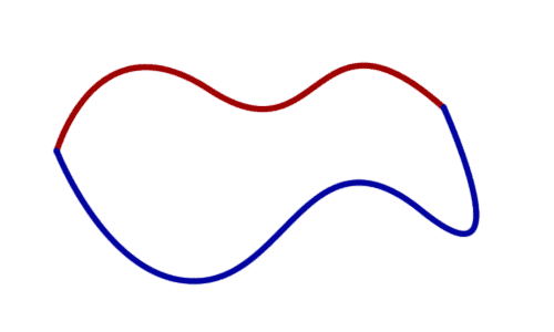
We can continuously transform the red path into the blue path; these two paths are homotopic.
On the other hand, if there is a hole in the space, as shown by the black disk below, no way to slide the red path to the blue path can be continuous; it would need to “jump” over the hole, which is a non-continuous operation. Indeed, no matter how small this hole is we can never overcome this problem; even if just a single point is missing, the nature of continuity ensures it.
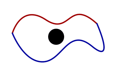
The black 'hole' in this plane makes it so the red path cannot be continuously transformed into the blue path; these paths are not homotopic.
In order to make this rigorous, we need to define a “path of paths,” so to speak. That is, we need a continuously parameterized family of continuous maps which for the parameter 0 gives the first path, and for 1 the second path.
Definition: Let $ f, g: [0,1] \to X$ be two paths in $ X$ with the same endpoints. A homotopy from $ f$ to $ g$ is a family of paths $ H_s: [0,1] \to X$ such that the following properties hold:
- $ H_0 = f$ as paths in $ X$
- $ H_1 = g$ as paths in $ X$
- For all $ s$, the path $ H_s(t)$ has the same endpoints as $ f$ and $ g$.
- $ H_s(t)$ is continuous in $ s$ and $ t$ simultaneously
If there is a homotopy between two paths, we call the two paths homotopic, and denote the relationship $ f \simeq g$.
We often think of $ s$ as the time variable, describing how far along we are in the transformation from $ f$ to $ g$. Here is a nice animation showing a homotopy of two paths:

A homotopy of paths, credit Wikipedia.
But don’t be fooled by the suggestive nature of these paths. While it will often be the case that two paths which are homeomorphic as topological spaces in themselves (viewed as subspaces of $ X$) will be homotopic, this is neither a sufficient nor a necessary condition for a homotopy to exist. Indeed, one can come up with a homotopy between a simple curve and a non simple curve, but these are not homeomorphic spaces (one has a cut-point). And in our picture above we give an example of two simple curves which are not homotopic: there is a hole in $ X$ that stops them from being so. So the existence of a homotopy depends almost entirely on the space that the paths are in, and on where the paths are in that space. This is good, because in the end we don’t care about the paths. We just care about what they tell us about $ X$.
Often times we will not need to give explicit homotopies; they can be quite complicated to construct. But here’s one widely used example: let us take two paths $ f,f’$ in the Euclidean plane from $ a$ to $ b$. Then we can construct the straight line homotopy between them as follows. Set $ H_s(t) = sf(t) + (1-s)f'(t)$. For $ s=0$ we get the path $ f'(t)$; for $ s=1$ we get the path $ f$; and for any fixed value of $ s$ we get a path from $ a$ to $ b$ (plug in $ t=0,1$ and verify the endpoints agree, and that the function is continuous in both variables). This example shows that all paths with the same endpoints in $ \mathbb{R}^2$ are homotopic. The same is true of $ \mathbb{R}^n$ in general, and we will use this fact later.
Because every path is homotopic to itself (the constant homotopy $ H_s(t) = f(t)$ for all $ s$), homotopy is symmetric ($ H_{-s}(t)$ gives an inverse homotopy $ g$ to $ f$), and homotopy is transitive (given in the parenthetical below), homotopy becomes an equivalence relation on paths in $ X$. So we may speak of the equivalence class of a path $ f$ as the set of all paths homotopic to it.
(Transitivity: given homotopies $ H_s(t)$ and $ G_{s}(t)$ from $ f \to g \to h$, we can construct a homotopy from $ f \to h$ as follows. The main difficulty is that the variable in our homotopy must go from 0 to 1, and so we cannot directly compose $ H$ and $ G$. Instead, we “run $ H$ twice as fast” and then “run $ G$ twice as fast.” That is, we define $ \Phi_s(t)$ piecewise to be $ H_{2s}(t)$ when $ s \in [0,1/2]$ and $ G_{2s-1}(t)$ when $ s \in [1/2, 1]$. The composition of continuous functions is continuous, so changing the $ s$ variable doesn’t break continuity. Moreover, since at time $ s=1/2$ the homotopies $ G,H$ coincide, and elsewhere they are continuous, we preserve continuity everywhere.)
This equivalence relation is precisely what we’ll use to define the existence of a hole. Intuitively speaking, if two paths with the same endpoints are not homotopic to each other, then there must be some obstruction stopping the homotopy. Then the number of distinct equivalence classes of paths with fixed endpoints will count the number of holes (plus one). Because endpoints are a little bit messy (one has to pick $ n+1$ endpoints for $ n$ non-equivalent paths to count $ n-1$ holes), we instead implement this idea with loops.
Definition: A path $ f:[0,1] \to X$ is a loop if $ f(0)=f(1)$. Since the two endpoints of a loop are the same, we call it the basepoint.
With loops or with paths, we need one more additional operation. The operation is called path composition, but it essentially “doing one path after the other.” That is, let $ f, g$ be paths in $ X$ such that $ f(1) = g(0)$. Then to compose $ g$ after $ f$, denoted via juxtaposition $ gf$, is the path defined by $ gf(t) = f(2t)$ when $ t \in [0,1/2]$ and $ gf(t) = g(2t-1)$ when $ t \in [1/2, 1]$. The same argument for “composing” homotopies works here: we run along $ f$ at twice the normal speed and then $ g$ at twice its normal speed to get $ gf$.
And now we turn to the main theorem of this post.
The Fundamental Group
Instead of looking at paths, we will work with loops with a fixed basepoint. The amazing thing that happens is that the set of equivalence classes of loops (with respect to homotopy) forms a group.
Definition: Let $ X$ be a topological space and fix a point $ x_0 \in X$. Define by $ \pi_1(X,x_0)$ the set of equivalence classes of loops with basepoint $ x_0$. This set is called the fundamental group of $ X$ (although we have not yet proved it is a group), or the first homotopy group of $ X$.
Theorem: The fundamental group is a group with respect to the operation of path composition.
Proof. In order to prove this we must verify the group operations. Let’s recall them here:
- The group must be closed under the group operation: clearly the composition of two loops based at $ x_0$ is again a loop at $ x_0$, but we need to verify this is well-defined. That is, the operation gives the same value regardless of which representative we choose from the equivalence class.
- The group operation must be associative.
- The group must have an identity element: the constant path $ t \mapsto x_0$ will fill this role.
- Every element must have an inverse: we will show that the loop which “runs in reverse” will serve this purpose.
To prove the first point, let $ f, g$ be loops, and suppose $ f’, g’$ are homotopic to $ f,g$ respectively. Then it should be the case that $ fg$ is homotopic to $ f’g’$. Suppose that $ H^1, H^2$ are homotopies between relevant loops. Then we can define a new homotopy which runs the two homotopies simultaneously, and composes their paths for any fixed $ s$. This is almost identical to the original definition of a path composition, since we simply need to define our new family of loops $ H$ by composing the loops $ H^1_s$ and $ H^2_s$. That is,
$ H_s(t) = H^1_s(2t)$ for $ t \in [0,1/2]$ and
$$H_s(t) = H^2_s(2t-1)$ for $ t \in [1/2, 1]$$So the operation is well-defined on equivalence classes.
Associativity is messier to prove, but has a similar mechanic. We just need to define a homotopy which scales the speed of each of the paths for a fixed $ s$ to be in sync. We omit the details for brevity.
For the identity, let $ f$ be a path and $ e$ denote the constant path at $late x_0$. Then we must find a homotopy from $ ef$ to $ f$ and $ fe$ to $ f$. Since the argument is symmetric we prove the former. The path $ ef$ sits at $ x_0$ for half of the time $ t \in [0,1]$ and performs $ f$ at twice speed for the rest. All we need to do is “continuously move” the time at which we stop $ e$ and start $ f$ from $ t=1/2$ to $ t=0$, and run $ f$ faster for the remaining time. We can equivalently perform this idea backwards (the algebra is simpler) to get
$ H_s(t) = x_0$ for $ t \in [0, s/2]$, and $ H_s(t) = f((2t-s)/(2-s))$ for $ t \in [s/2, 1]$.
To verify this works, plugging in $ s=0$ gives precisely the definition of the composition $ ef$, and for $ s=1$ we recover $ f(t)$. Moreover for any value of $ s$ setting $ t=0$ gives $ x_0$ and $ t=1$ gives $ f(1)$. Finally, the point at which the two pieces meet is $ t = s/2$, and we only need verify that the piecewise definition agrees there. That is, the argument of $ f$ must be zero for that value of $ t$ regardless of the choice of $ s$. Indeed it is.
Finally, for inverses define $ f^-(t) = f(1-t)$ to be the “reverse path” of $ f$. Now we simply need to prove that $ ff^-$ is homotopic to $ e$. That is, we need to run $ f$ part way, and then run $ f^-$ starting from that spot in the reverse direction. The point at which we stop to turn back is $ t=(1-s)$, which continuously moves from $ t=1$ to $ t=0$. We leave the formal specification of this homotopy as an exercise to the reader (hint: we need to appropriately change the speed at which $ f, f^-$ run in order to make everything fit together). From here on we will identify the two notations $ f^{-1} = f^-$ as homotopy equivalence classes of paths. $ \square$
The high-level implications of this theorem are quite important. Although we have not proved it here, the fundamental group is a topological invariant. That is, if $ X$ and $ Y$ are two topological spaces, $ x_0 \in X, y_0 \in Y$, and there is an isomorphism $ f:X \to Y$ which takes $ x_0 \mapsto y_0$, then $ \pi_1(X,x_0) \cong \pi_1(Y,y_0)$ are isomorphic as groups. That is (and this is the important bit) if $ X$ and $ Y$ have different fundamental groups, then we know immediately that they cannot be homeomorphic. The way to prove this is to use $ f$ to construct a new induced homomorphism of groups and proving that it is an isomorphism. We give a description of this in the next section.
In fact, we can say something stronger: the fundamental group is a homotopy invariant. That is, we can generalize the idea of a path homotopy into a “homotopy of maps,” and say that two spaces $ X, Y$ are homotopy equivalent if there are maps $ f: X \to Y, g: Y \to X$ with $ fg \simeq \textup{id}_Y$ (the identity function on $ Y$) and $ gf \simeq \textup{id}_X$. The important fact is that two spaces which are homotopy equivalent necessarily have isomorphic fundamental groups. It should also be clear that homeomorphic spaces are homotopy equivalent (the homeomorphism map is also a homotopy equivalence map), so this realizes the fundamental group as a topological invariant as well. We will not prove this here, and instead refer to Hatcher, Chapter 1.
An important example of two spaces which are homotopy equivalent but not homeomorphic is that of the Möbius band and the circle. Proving it requires some additional tools we haven’t covered on this blog, but the idea is that one can squeeze the Möbius strip down onto its center circle, and so the loops in the former correspond to loops in the latter. So the Möbius band also has fundamental group $ \mathbb{Z}$.
Additionally, if the space $ X$ is path-connected, then the choice of a basepoint is irrelevant. A sketch of the proof goes as follows: let $ x_0, x_1$ be two choices of basepoints, and pick a path $ p$ from $ x_0$ to $ x_1$. Then we can naturally take any loop $ f$ based at $ x_1$ to a corresponding loop at $ x_0$ by composing $ p^-fp$ as in the following picture (here we traverse the paths in left-to-right order, which is the opposite of how function composition usually works; this is so we can read the paths from left-to-right in the order they are traversed in the diagram).
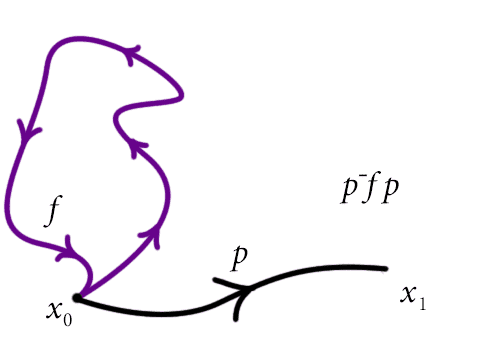
An example of a change of basepoint map.
More rigorously this operation induces a homomorphism on the fundamental group (we define this fully in the next section), and for path connected spaces this is an isomorphism of groups. And so we can speak of the fundamental group $ \pi_1(X)$ when we work with sufficiently nice spaces (and in practice we always will).
Computing Fundamental Groups
So now we have seen that the fundamental group is in fact a group, but how can we compute it? Groups can be large and wild, and so can topological spaces. So it’s really impressive that we can compute these groups at all.
First off, the simplest possibility is that the fundamental group of $ X$ is the identity group. That is, that every loop is homotopic to the trivial loop. In this case we call $ X$ simply connected. For example, Euclidean space is simply connected. We gave the proof above showing that any two paths with the same endpoints in $ \mathbb{R}^2$ are homotopic, and the proof is the same in general. Since all loops are homotopic to each other, they are all homotopic to the trivial loop, and so $ \pi_1(\mathbb{R}^n) = 1$ is the trivial group. The picture becomes more interesting when we start to inspect subspaces of Euclidean space with nontrivial holes in them.
In fact, the first nontrivial fundamental group one computes in developing this theory is that of the circle $ \pi_1(S^1) = \mathbb{Z}$. We again defer the proof to Hatcher because it is quite long, but the essential idea is as follows. View the circle as a subset of the complex plane $ \mathbb{C}$, and fix the basepoint $ x_0 = 1$. The only distinct kinds of loops are those loops which loop around the circle $ n$ times clockwise, or $ n$ times counterclockwise, where $ n \in \mathbb{Z}$ is arbitrary. That is, we can construct a function $ f: \mathbb{Z} \to \pi_1(S^1)$ sending $ n$ to the loop $ t \mapsto e^{2 \pi i nt}$ which goes $ n$ times around the circle (negative $ n$ make it go in the negative direction). This map is an isomorphism.
From this one computation we get quite a few gains. As we will see in a moment, many fundamental groups are free products of $ \mathbb{Z}$ with added relators, and the upcoming van Kampen theorem tells us how these relators are determined. On the other hand, we have already seen on this blog that the fundamental group of the circle is powerful enough to prove the fundamental theorem of algebra! It is clear from this that $ \pi_1$ is a powerful notion.
Let’s take a moment to interpret this group in terms of the number of “holes” of $ S^1$. There may be some confusion because this group is infinite, but there is only one hole. Indeed, for each “hole” of a space one would expect to get a copy of $ \mathbb{Z}$, since one may run a loop arbitrarily many times around that hole in either clockwise or counterclockwise direction. Recall the classification theorem for finitely generated abelian groups from our recent primer. Since every such abelian group decomposes into a finite number of copies of $ \mathbb{Z}$ and a torsion part, then we should be interpreting the number of holes of $ X$ as the rank of $ \pi_1(X)$ (the number of copies of $ \mathbb{Z}$).
This is great! But unfortunately nothing guarantees that the fundamental group is abelian, and for more complicated spaces things aren’t even so simple in the abelian case. In a moment, we will see an example of a space with a nonabelian fundamental group (in fact, we’ve already seen this space on this blog). One of its pieces will be $ \mathbb{Z}/2\mathbb{Z}$. So our interpretation would say that this space has no holes in it, but what does the extra torsion factor mean? As it turns out the specific factor $ \mathbb{Z}/2\mathbb{Z}$ happens to correspond to non-orientability.
In fact it is true that for every group $ G$, there is a two-dimensional topological space whose fundamental group is $ G$ (we haven’t defined dimension yet, but the notion of a surface is intuitive enough). So any weird torsion factor shows up in the fundamental group of some sufficiently awkward space. When one starts to investigate more and more of these contrived spaces, one ceases to care about the “intuitive” interpretations of the fundamental group. The group simply becomes a topological invariant, and the extra factors are just extra ways to tell spaces apart.
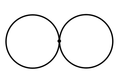
We want to state a powerful tool for computing fundamental groups whose rigorous version is called the van Kampen theorem. The intuition is as follows. Imagine we have a so-called “wedge” of two circles.
wedge
From our intuition of this space as two copies of a circle, we would expect its fundamental group to be $ \mathbb{Z}^2$. Unfortunately it is not, because we can immediately see that the fundamental group of this space is not commutative. In particular, let us label the loops $ a$ and $ b$, and give them orientation:

wedge-with-labels
Then the loop $ ab$ (we traverse these loops in left-to-right order for ease of reading) is not homotopic to the loop $ ba$. Instead, this group should be the free group on the generators $ a, b$. Recall from our second primer on group theory that this means the two generators have no nontrivial relations between them. The reason it is free is because the intersection of the two circles (whose fundamental groups we know separately) is simply connected. If it were not, then there would be some relations. For instance, let us look at the torus $ X = T^1$, and recall its formulation as a quotient of a disk.
torus-quotient
Here the two top edges and sides are identified, and so we can label the loops as follows:

torus
Then the boundary of the original disk is just $ aba^{-1}b^{-1}$. Since any loop bounding a disk is homotopic to a constant loop (the straight line homotopy works here), we see that the loop $ aba^{-1}b^{-1} = 1$ in $ \pi_1(X)$. That is, we still have two generators $ a,b$ corresponding to the longitudinal and latitudinal circles, but traversing them in the right order is the same as doing nothing. This youtube video gives an animation showing the homotopy in action. So the fundamental group of the torus has presentation:
$$\displaystyle G = \left \langle a,b | aba^{-1}b^{-1} = 1 \right \rangle$$This is obviously just $ \mathbb{Z}^2$, since the defining relation is precisely saying that the two generators commute: $ ab=ba$. That is, it is the free abelian group on two generators.
Before we can prove the theorem in general we need to define an induced homomorphism. Given two spaces $ X, Y$ and a map $ f: X \to Y$, one gets a canonical induced map $ f^*: \pi_1(X) \to \pi_1(Y)$. If we consider basepoints, then we also require that $ f$ preserves the basepoint. The induced map is defined by setting $ f^*(p)$ to be the equivalence class of the loop $ fp$ of $ Y$. Recalling that $ fp$ is indeed a loop whenever $ f$ is continuous, it is not hard to see that this is a homomorphism of groups. It is certainly not in general an isomorphism; for instance the trivial map which sends all of $ X$ to a single point will not preserve nontrivial loops. But as we will see in the van Kampen theorem, for some maps it is.
One interesting example of an induced homomorphism is that of the inclusion map. Let $ Y \subset X$ be a subspace, and let $ i: Y \hookrightarrow X$ be the inclusion map $ i(y) = y$. This will often not induce an isomorphism $ i^*$ on fundamental groups. For example, the inclusion of $ S^1 \hookrightarrow \mathbb{R}^2$ is not a constant map, but it induces the constant map on fundamental groups since there is only one group homomorphism from any group to the trivial group $ \mathbb{Z} \to 1$. That is, the kernel of $ i^*$ is all of $ \mathbb{Z}$. Intuitively we are “filling in” the hole in $ S^1$ with the ambient space from $ \mathbb{R}^2$ so that the loop generating $ \mathbb{Z}$ is homotopic to the trivial loop. Thus, we are killing all of the loops of the circle.
The more important remark for the van Kampen theorem is, recalling our primer on group theory, that any collection of homomorphisms on groups $ \varphi_{\alpha} : G_{\alpha} \to H$ extends uniquely to a homomorphism on the free product $ \varphi: \ast_{\alpha} G_{\alpha} \to H$. The main goal of this theorem is to give us a way to build up fundamental groups in the same way we build up topological spaces. And it does so precisely by saying that this $ \varphi$ map on the free product is surjective. Using the first isomorphism theorem (again see our primer), this will allow us to compute the fundamental group of a space $ X$ given subspaces $ A_{\alpha}$ and by analyzing the kernels of the homomorphisms induced by the inclusions $ i_{\alpha}: A_{\alpha} \to X$.
The last thing we need to set up this theorem is a diagram. If we have two subspaces $ A_{\alpha}, A_{\beta}$ and we look at the inclusion $ i: A_{\alpha} \cap A_{\beta} \to X$, we could define it in one of two equivalent ways: first by going through $ A_{\alpha}$ and then to $ X$, or else by going through $ A_{\beta}$ first. The diagram is as follows:
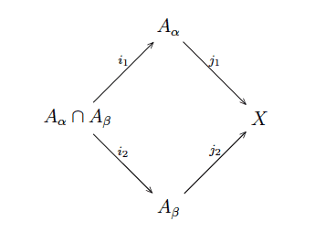
inclusion-diagram
However, the induced homomorphism will depend on this choice! So we denote $ i_1^* : A_{\alpha} \cap A_{\beta} \to A_{\alpha}$ to include into the first piece, and $ i_2^*$ to include on the second piece $ A_{\beta}$. The diagram here is:
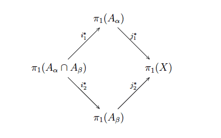
inclusion-diagram-pi1
Now we can state the theorem (and it is still quite a mouthful).
Theorem: (van Kampen) Let $ X$ be the union of a family of path-connected open subspaces $ A_{\alpha}$, each of which contains the chosen basepoint $ x_0 \in X$. Let $ i_{\alpha}: A_{\alpha} \to X$ be inclusions, $ i_{\alpha}^*$ the induced homomorphisms, and $ \varphi$ the unique extension of the inclusion $ i_{\alpha}^*$ to the free product $ \ast_{\alpha} \pi_1(A_{\alpha}, x_0)$.
- If all intersections of pairs $ A_{\alpha} \cap A_{\beta}$ are path-connected, then $ \varphi$ is a surjection.
- If in addition all triple intersections $ A_{\alpha} \cap A_{\beta} \cap A_{\gamma}$ are path-connected, then the kernel of $ \varphi$ is the smallest normal subgroup $ N$ generated by the elements $ i_1^*(x)i_2^*(x)^{-1}$ for $ x \in \pi_1(A_{\alpha} \cap A_{\beta})$.
In particular, the first isomorphism theorem gives an isomorphism $ \ast \pi_1(A_{\alpha}) / N \cong \pi_1(X)$. That is, we can compute the fundamental group of $ X$ by knowing the fundamental groups of the pieces $ A_{\alpha}$ and a little bit of extra information.
We do not have the stamina to prove such a massive theorem on this blog. However, since we have done so much just to state it, we would be cheating the reader by omitting any examples of its usage.
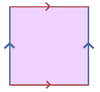
Let’s again look at the torus $ T^1$. Viewing it as in our previous primer on constructing topological spaces, it is the following quotient of a disk:
torus-quotient
Split the disk into two subspaces $ A,B$ as follows:

torus-van-kampen
Note how these spaces overlap in an annulus whose fundamental group we’ve already seen is $ \mathbb{Z}$. Moreover, the fundamental group of $ A$ is trivial, and the fundamental group of $ B$ is $ \mathbb{Z} \ast \mathbb{Z} = \left \langle a,b \right \rangle$. To see the latter, note that the torus with a disk removed is homotopy equivalent to a wedge of two circles. A simple exercise (again using the van Kampen theorem) finishes the computation of $ \pi_1(B)$. As we said, the intersection $ A \cap B$ has fundamental group $ \mathbb{Z} = \left \langle c \right \rangle$ (it is just an annulus).
So according to the van Kampen theorem, the fundamental group of $ T^1$ is the free group on two generators, modulo the normal subgroup found by identifying the images of the two possible induced homomorphisms $ \pi_1(A \cap B) \hookrightarrow \pi_1(X)$. On one hand the image going through $ \pi_1(A)$ is trivial because the group itself is trivial. On the other hand the image going through $ \pi_1(B)$ is easily seen to be homeomorphic to an oriented traversal of the boundary path $ aba^{-1}b^{-1}$. Indeed, this gives rise to a single relator: $ aba^{-1}b^{-1} = 1$. So this verifies the presentation we gave for the fundamental group of the torus above.
A nearly identical argument gives nearly identical presentations for the Klein bottle. There is a slightly different presentation for the real projective plane, and it is interesting because there is a topological hole, but the group is just $ \mathbb{Z}/2\mathbb{Z}$. We leave this as an exercise to the reader, using the representation as a quotient of the disk provided in our previous primer.
Our second example is that of the n-sphere $ S^n$. We already know $ \pi_1(S^1) = \mathbb{Z}$, but in fact $ \pi_1(S^n)$ is trivial for all larger $ n$. Inductively, we can construct $ S^n$ from two copies of the open ball $ B^n$ by taking one to be the northern hemisphere, one to be the southern hemisphere, and their intersection to be the equator (or rather, something homotopy equivalent to $ S^{n-1}$).
For the case of $ S^2$, we have that each hemisphere is an open ball centered at the poles (though the center is irrelevant), and the intersection is an annulus which is homotopy equivalent to $ S^1$. Each of the two pieces is simply connected (in fact, homeomorphic to $ \mathbb{R^n}$), and so by van Kampen’s theorem the fundamental group of $ S^2$ is the free product of two trivial groups (modulo the trivial subgroup), and is hence the trivial group.
This argument works in general: if we know that each of the $ D^n$ have trivial fundamental groups, and each of the possible intersections $ S^{n-1}$ are path-connected (which is easy to see by looking at the construction via a simplicial complex), then van Kampen’s theorem guarantees that the fundamental group of $ S^n$ is trivial.
So as we have seen, the fundamental group is a nice way to compute the number (or the structure) of the one-dimensional holes of a topological space. Unfortunately, even for the nicest of spaces (simplicial complexes) the problem of computing fundamental groups is in general undecidable. In fact, we get stuck at a simpler problem. The problem of determining whether the fundamental group of a finite simplicial complex is trivial is undecidable.
That is, for programmers the fundamental group is practically useless, though there are some special cases.
Higher Homotopy Groups
There is an obvious analogue for 2-, 3-, and n-dimensional holes. That is, we can define the $ n$-th homotopy group of a space $ X$, denoted $ \pi_n(X)$ to be the set of homotopy equivalence classes of maps $ S^n \to X$. Homotopy groups $ \pi_n(X)$ for $ n > 1$ are called higher homotopy groups.
As one would expect, higher homotopy groups are much more difficult and even harder to compute. In fact, the only reason we bring this up in this primer is to intimidate the reader: we don’t even know a general way to compute the higher homotopy groups of the sphere.
In particular, here is a table of the known higher homotopy groups of the sphere.

The known higher homotopy groups of spheres. Taken from Wikipedia
The thick black line shows the boundary between where the patterns are well-known and understood (below) and the untamed wilderness (above). This table solidifies how ridiculous the higher homotopy groups can be. As such, they are unsuitable for computational purposes.
Nevertheless, the homotopy groups are relatively easy to understand in terms of intuition, because a homotopy is easily visualized. In our next primer, we will trade this ease of intuition for ease of computation. In particular, we will develop the notion of a homology group, and for simplicial complexes their computation will be about as simple as matrix reduction.
Once this is done, we will extend the idea of homology to apply to data sets (which should not themselves be considered as topological spaces), and we will be able to compute the topological features of a data set. This is our ultimate goal, but the mathematics we lay down along the way will have their own computational problems that we can explore on this blog.
Until next time!
Want to respond? Send me an email, post a webmention, or find me elsewhere on the internet.