A common problem in machine learning is to take some kind of data and break it up into “clumps” that best reflect how the data is structured. A set of points which are all collectively close to each other should be in the same clump.
A simple picture will clarify any vagueness in this:
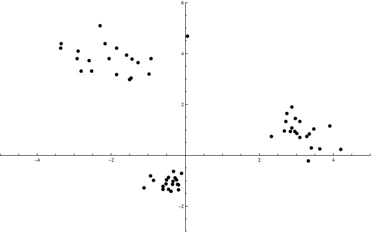
cluster-example
Here the data consists of points in the plane. There is an obvious clumping of the data into three pieces, and we want a way to automatically determine which points are in which clumps. The formal name for this problem is the clustering problem. That is, these clumps of points are called clusters, and there are various algorithms which find a “best” way to split the data into appropriate clusters.
The important applications of this are inherently similarity-based: if our data comes from, say, the shopping habits of users of some website, we may want to target a group of shoppers who buy similar products at similar times, and provide them with a coupon for a specific product which is valid during their usual shopping times. Determining exactly who is in that group of shoppers (and more generally, how many groups there are, and what the features the groups correspond to) if the main application of clustering.
This is something one can do quite easily as a human on small visualizable datasets, but the usual the digital representation (a list of numeric points with some number of dimensions) doesn’t yield any obvious insights. Moreover, as the data becomes more complicated (be it by dimension increase, data collection errors, or sheer volume) the “human method” can easily fail or become inconsistent. And so we turn to mathematics to formalize the question.
In this post we will derive one possible version of the clustering problem known as the k-means clustering or centroid clustering problem, see that it is a difficult problem to solve exactly, and implement a heuristic algorithm in place of an exact solution.
And as usual, all of the code used in this post is freely available on this blog’s Github page.
Partitions and Squared Deviations
The process of clustering is really a process of choosing a good partition of the data. Let’s call our data set $ S$, and formalize it as a list of points in space. To be completely transparent and mathematical, we let $ S$ be a finite subset of a metric space $ (X,d)$, where $ d$ is our distance metric.
Definition: We call a partition of a set $ S$ a choice of subsets $ A_1, \dots, A_n$ of $ S$ so that every element of $ S$ is in exactly one of the $ A_i$.
A couple of important things to note about partitions is that the union of all the $ A_i$ is $ S$, and that any two $ A_i, A_j$ intersect trivially. These are immediate consequences of the definition, and together provide an equivalent, alternative definition for a partition. As a simple example, the even and odd integers form a partition of the whole set of integers.
There are many different kinds of clustering problems, but every clustering problem seeks to partition a data set in some way depending on the precise formalization of the goal of the problem. We should note that while this section does give one of many possible versions of this problem, it culminates in the fact that this formalization is too hard to solve exactly. An impatient reader can safely skip to the following section where we discuss the primary heuristic algorithm used in place of an exact solution.
In order to properly define the clustering problem, we need to specify the desired features of a cluster, or a desired feature of the set of all clusters combined. Intuitively, we think of a cluster as a bunch of points which are all close to each other. We can measure this explicitly as follows. Let $ A$ be a fixed subset of the partition we’re interested in. Then we might want to optimize the sum of all of the distances of pairs of points within $ A$ to be a measure of it’s “clusterity.” In symbols, this would be
$$\displaystyle \sum_{x \neq y \in A} d(x, y)$$If this quantity is small, then it says that all of the points in the cluster $ A$ are close to each other, and $ A$ is a good cluster. Of course, we want all clusters to be “good” simultaneously, so we’d want to minimize the sum of these sums over all subsets in the partition.
Note that if there are $ n$ points in $ A$, then the above sum involves $ \choose{n}{2} \sim n^2$ distance calculations, and so this could get quite inefficient with large data sets. One of the many alternatives is to pick a “center” for each of the clusters, and try to minimize the sum of the distances of each point in a cluster from its center. Using the same notation as above, this would be
$$\displaystyle \sum_{x \in A} d(x, c)$$where $ c$ denotes the center of the cluster $ A$. This only involves $ n$ distance calculations, and is perhaps a better measure of “clusterity.” Specifically, if we use the first option and one point in the cluster is far away from the others, we essentially record that single piece of information $ n – 1$ times, whereas in the second we only record it once.
The method we will use to determine the center can be very general. We could use one of a variety of measures of center, like the arithmetic mean, or we could try to force one of the points in $ A$ to be considered the “center.” Fortunately, the arithmetic mean has the property that it minimizes the above sum for all possible choices of $ c$. So we’ll stick with that for now.
And so the clustering problem is formalized.
Definition: Let $ (X,d)$ be a metric space with metric $ d$, and let $ S \subset (X,d)$ be a finite subset. The centroid clustering problem is the problem of finding for any positive integer $ k$ a partition $ \left \{ A_1 ,\dots A_k \right \}$ of $ S$ so that the following quantity is minimized:
$$\displaystyle \sum_{i=1}^k\sum_{x \in A_i} d(x, c(A_i))$$where $ c(A_i)$ denotes the center of a cluster, defined as the arithmetic mean of the points in $ A_i$:
$$\displaystyle c(A) = \frac{1}{|A|} \sum_{x \in A} x$$Before we continue, we have a confession to make: the centroid clustering problem is prohibitively difficult. In particular, it falls into a class of problems known as NP-hard problems. For the working programmer, NP-hard means that there is unlikely to be an exact solution to the problem which is better than trying all possible partitions.
We’ll touch more on this after we see some code, but the salient fact is that a heuristic algorithm is our best bet. That is, all of this preparation with partitions and squared deviations really won’t come into the algorithm design at all. Formalizing this particular problem in terms of sets and a function we want to optimize only allows us to rigorously prove it is difficult to solve exactly. And so, of course, we will develop a naive and intuitive heuristic algorithm to substitute for an exact solution, observing its quality in practice.
Lloyd’s Algorithm
The most common heuristic for the centroid clustering problem is Lloyd’s algorithm, more commonly known as the k-means clustering algorithm. It was named after its inventor Stuart Lloyd, a University of Chicago graduate and member of the Manhattan project who designed the algorithm in 1957 during his time at Bell Labs.
Heuristics tend to be on the simpler side, and Lloyd’s algorithm is no exception. We start by fixing a number of clusters $ k$ and choosing an arbitrary initial partition $ A = \left \{ A_1, \dots, A_k \right \}$. The algorithm then proceeds as follows:
repeat:
   compute the arithmetic mean c[i] of each A[i]
   construct a new partition B:
      each subset B[i] is given a center c[i] computed from A
      x is assigned to the subset B[i] whose c[i] is closest
   stop if B is equal to the old partition A, else set A = B
Intuitively, we imagine the centers of the partitions being pulled toward the center of mass of the points in its currently assigned cluster, and then the points deciding selectively who to pull towards them. (Indeed, precisely because of this the algorithm may not always give sensible results, but more on that later.)
One who is in tune with their inner pseudocode will readily understand the above algorithm. But perhaps the simplest way to think about this algorithm is functionally. That is, we are constructing this partition-updating function $ f$ which accepts as input a partition of the data and produces as output a new partition as follows: first compute the mean of centers of the subsets in the old partition, and then create the new partition by gathering all the points closest to each center. These are the fourth and fifth lines of the pseudocode above.
Indeed, the rest of the pseudocode is merely pomp and scaffolding! What we are really after is a fixed point of the partition-updating function $ f$. In other words, we want a partition $ P$ such that $ f(P) = P$. We go about finding one in this algorithm by applying $ f$ to our initial partition $ A$, and then recursively applying $ f$ to its own output until we no longer see a change.
Perhaps we should break away from traditional pseudocode illegibility and rewrite the algorithm as follows:
define updatePartition(A):
   let c[i] = center(A[i])
   return a new partition B:
      each B[i] is given the points which are closest to c[i]

compute a fixed point by recursively applying
updatePartition to any initial partition.
Of course, the difference between these pseudocode snippets is just the difference between functional and imperative programming. Neither is superior, but the perspective of both is valuable in its own right.
And so we might as well implement Lloyd’s algorithm in two such languages! The first, weighing in at a whopping four lines, is our Mathematica implementation:
closest[x_, means_] :=
  means[[First[Ordering[Map[EuclideanDistance[x, #] &, means]]]]];

partition[points_, means_] := GatherBy[points, closest[#, means]&];
updatePartition[points_, old_] := partition[points, Map[Mean, old]];

kMeans[points_, initialMeans_] := FixedPoint[updatePartition[points, #]&, partition[points, initialMeans]];
While it’s a little bit messy (as nesting 5 function calls and currying by hand will inevitably be), the ideas are simple. The “closest” function computes the closest mean to a given point $ x$. The “partition” function uses Mathematica’s built-in GatherBy function to partition the points by the closest mean; GatherBy[L, f] partitions its input list L by putting together all points which have the same value under f. The “updatePartition” function creates the new partition based on the centers of the old partition. And finally, the “kMeans” function uses Mathematica’s built-in FixedPoint function to iteratively apply updatePartition to the initial partition until there are no more changes in the output.
Indeed, this is as close as it gets to the “functional” pseudocode we had above. And applying it to some synthetic data (three randomly-sampled Gaussian clusters that are relatively far apart) gives a good clustering in a mere two iterations:
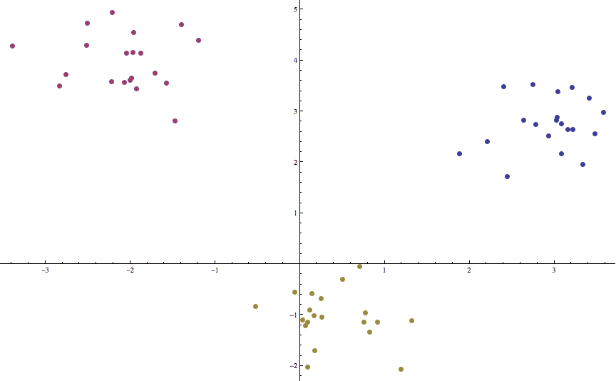
k-means-example
Indeed, we rarely see a large number of iterations, and we leave it as an exercise to the reader to test Lloyd’s algorithm on random noise to see just how bad it can get (remember, all of the code used in this post is available on this blog’s Github page). One will likely see convergence on the order of tens of iterations. On the other hand, there are pathologically complicated sets of points (even in the plane) for which Lloyd’s algorithm takes exponentially long to converge to a fixed point. And even then, the solution is never guaranteed to be optimal. Indeed, having the possibility for terrible run time and a lack of convergence is one of the common features of heuristic algorithms; it is the trade-off we must make to overcome the infeasibility of NP-hard problems.
Our second implementation was in Python, and compared to the Mathematica implementation it looks like the lovechild of MUMPS and C++. Sparing the reader too many unnecessary details, here is the main function which loops the partition updating, a la the imperative pseudocode:
def kMeans(points, k, initialMeans, d=euclideanDistance):
   oldPartition = []
   newPartition = partition(points, k, initialMeans, d)

   while oldPartition != newPartition:
      oldPartition = newPartition
      newMeans = [mean(S) for S in oldPartition]
      newPartition = partition(points, k, newMeans, d)

   return newPartition
We added in the boilerplate functions for euclideanDistance, partition, and mean appropriately, and the reader is welcome to browse the source code for those.
Birth and Death Rates Clustering
To test our algorithm, let’s apply it to a small data set of real-world data. This data will consist of one data point for each country consisting of two features: birth rate and death rate, measured in annual number of births/deaths per 1,000 people in the population. Since the population is constantly changing, it is measured at some time in the middle of the year to act as a reasonable estimate to the median of all population values throughout the year.
The raw data comes directly from the CIA’s World Factbook data estimate for 2012. Formally, we’re collecting the “crude birth rate” and “crude death rate” of each country with known values for both (some minor self-governing principalities had unknown rates). The “crude rate” simply means that the data does not account for anything except pure numbers; there is no compensation for the age distribution and fertility rates. Of course, there are many many issues affecting the birth rate and death rate, but we don’t have the background nor the stamina to investigate their implications here. Indeed, part of the point of studying learning methods is that we want to extract useful information from the data without too much human intervention (in the form of ambient knowledge).
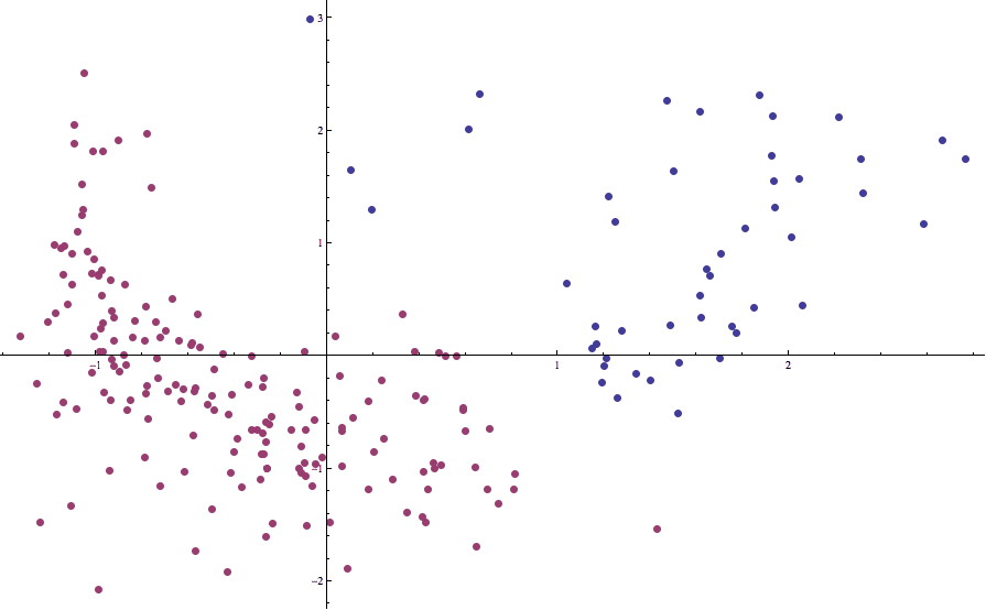
Here is a plot of the data with some interesting values labeled (click to enlarge):
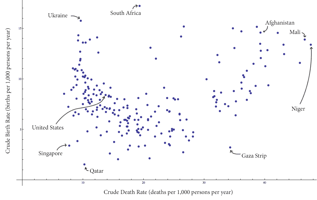
countries-birth-deat-labeled
Specifically, we note that there is a distinct grouping of the data into two clusters (with a slanted line apparently separating the clusters). As a casual aside, it seems that the majority of the countries in the cluster on the right are countries with active conflict.
Applying Lloyd’s algorithm with $ k=2$ to this data results in the following (not quite so good) partition:
countries-birth-death-unstandardized
Note how some of the points which we would expect to be in the “left” cluster are labeled as being in the right. This is unfortunate, but we’ve seen this issue before in our post on k-nearest-neighbors: the different axes are on different scales. That is, death rates just tend to vary more wildly than birth rates, and the two variables have different expected values.
Compensating for this is quite simple: we just need to standardize the data. That is, we need to replace each data point with its deviation from the mean (with respect to each coordinate) using the usual formula:
$$\displaystyle z = \frac{x – \mu}{\sigma}$$where for a random variable $ X$, its (sample) expected value is $ \mu$ and its (sample) standard deviation is $ \sigma$. Doing this in Mathematica is quite easy:
Transpose[Map[Standardize, Transpose[L]]]
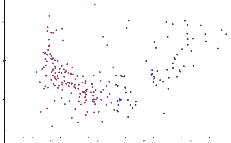
where L is a list containing our data. Re-running Lloyd’s algorithm on the standardized data gives a much better picture:
countries-birth-death-2cluster
Now the boundary separating one cluster from the other is in line with what our intuition dictates it should be.
Heuristics… The Air Tastes Bitter
We should note at this point that we really haven’t solved the centroid clustering problem yet. There is one glaring omission: the choice of $ k$. This question is central to the problem of finding a good partition; a bad choice can yield bunk insights at best. Below we’ve calculated Lloyd’s algorithm for varying values of $ k$ again on the birth-rate data set.
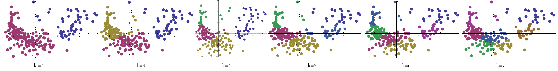
Lloyd's algorithm processed on the birth-rate/death-rate data set with varying values of k between 2 and 7.
The problem of finding $ k$ has been addressed by many a researcher, and unfortunately the only methods to find a good value for $ k$ are heuristic in nature as well. In fact, many believe that to determine the correct value of $ k$ is a learning problem in of itself! We will try not to go into too much detail about parameter selection here, but needless to say it is an enormous topic.
And as we’ve already said, even if the correct choice of $ k$ is known, there is no guarantee that Lloyd’s algorithm (or any algorithm attempting to solve the centroid clustering problem) will converge to a global optimum solution. In the same fashion as our posts on cryptoanalysis and deck-stacking in Texas Hold ‘Em, the process of finding a minimum can converge to a local minimum.
Here is an example with four clusters, where each frame is a step, and the algorithm progresses from left to right (click to enlarge):

One way to alleviate the issues of local minima is the same here as in our other posts: simply start the algorithm over again from a different randomly chosen starting point. That is, as in our implementations above, our “initial means” are chosen uniformly at random from among the data set points. Alternatively, one may randomly partition the data (without respect to any center; each data point is assigned to one of the $ k$ clusters with probability $ 1/k$). We encourage the reader to try both starting conditions as an exercise, and implement the repeated algorithm to return that output which minimizes the objective function (as detailed in the “Partitions and Squared Deviations” section).
And even if the algorithm will converge to a global minimum, it might not be the case that it does so efficiently. As we already mentioned, solving the problem of centroid clustering (even for a fixed $ k$) is NP-hard. And so (assuming $ \textup{P} \neq \textup{NP}$) any algorithm which converges to a global minimum will take exponentially long on some pathological inputs. The interested reader will see this exponentially slow convergence even in the case of k=2 for points in the plane (that is as simple as it gets).
These kinds of reasons make Lloyd’s algorithm and the centroid clustering problem a bit of a poster child of machine learning. In theory it’s difficult to solve exactly, but it has an efficient and widely employed heuristic used in practice which is often good enough. Moreover, since the exact solution is more or less hopeless, much of the focus has shifted to finding randomized algorithms which on average give solutions that are within some constant-factor approximation of the true minimum.
A Word on Expectation Maximization
This algorithm shares quite a bit of features with a very famous algorithm called the Expectation-Maximization algorithm. We plan to investigate this after we spend some more time on probability theory on this blog, but the (very rough) idea is that the algorithm operates in two steps. First, a measure of “center” is chosen for each of a number of statistical models based on given data. Then a maximization step occurs which chooses the optimal parameters for those statistical models, in the sense that the probability that the data was generated by statistical models with those parameters is maximized. These statistical models are then used as the “old” statistical models whose centers are computed in the next step.
Continuing the analogy with clustering, one feature of expectation-maximization that makes it nice is it allows the sizes of the “clusters” to have varying sizes, whereas Lloyd’s algorithm tends to make its clusters have equal size (as we saw with varying values of $ k$ in our birth-rates example above).
And so the ideas involved in this post are readily generalizable, and the applications extend to a variety of fields like image reconstruction, natural language processing, and computer vision. The reader who is interested in the full mathematical details can see this tutorial.
Until next time!