Last time we discussed the setup for the silent duel problem: two players taking actions in $ [0,1]$, player 1 gets $ n$ chances to act, player 2 gets $ m$, and each knows their probability of success when they act.
The solution is in a paper of Rodrigo Restrepo from the 1950s. In this post I’ll start detailing how I study this paper, and talk through my thought process for approaching a bag of theorems and proofs. If you want to follow along, I re-typeset the paper on Github.
Game Theory Basics
The Introduction starts with a summary of the setting of game theory. I remember most of this so I will just summarize the basics of the field. Skip ahead if you already know what the minimax theorem is, and what I mean when I say the “value” of a game.
A two-player game consists of a set of actions for each player—which may be finite or infinite, and need not be the same for both players—and a payoff function for each possible choice of actions. The payoff function is interpreted as the “utility” that player 1 gains and player 2 loses. If the payoff is negative, you interpret it as player 1 losing utility to player 2. Utility is just a fancy way of picking a common set of units for what each player treasures in their heart of hearts. Often it’s stated as money and we assume both players value cash the same way. Games in which the utility is always “one player gains exactly the utility lost by the other player” are called zero-sum.
With a finite set of actions, the payoff function is a table. For rock-paper-scissors the table is:
Rock, paper: -1
Rock, scissors: 1
Rock, rock: 0
Paper, paper: 0
Paper, scissors: -1
Paper, rock: 1
Scissors, paper: 1
Scissors, scissors: 0
Scissors, rock: -1
You could arrange this in a matrix and analyze the structure of the matrix, but we won’t. It doesn’t apply to our forthcoming setting where the players have infinitely many strategies.
A strategy is a possibly-randomized algorithm (whose inputs are just the data of the game, not including any past history of play) that outputs an action. In some games, the optimal strategy is to choose a single action no matter what your opponent does. This is sometimes called a pure, dominating strategy, not because it dominates your opponent, but because it’s better than all of your other options no matter what your opponent does. The output action is deterministic.
However, as with rock-paper-scissors, the optimal strategy for most interesting games requires each player to act randomly according to a fixed distribution. Such strategies are called mixed or randomized. For rock-paper-scissors, the optimal strategy is to choose rock, paper, and scissors with equal probability. Computers are only better than humans at rock-paper-scissors because humans are bad at behaving consistently and uniformly random.
The famous minimax theorem says that every two-player zero-sum game has an optimal strategy for each player, which is possibly randomized. This strategy is optimal in the sense that it maximizes your expected winnings no matter what your opponent does. However, if your opponent is playing a particularly suboptimal strategy, the minimax solution might not be as good as a solution that takes advantage of the opponent’s dumb choices. A uniform random rock-paper-scissors strategy is not optimal if your opponent always plays “rock.” However, the optimal strategy doesn’t need special knowledge or space to store information about past play. If you played against God, you would blindly use the minimax strategy and God would have no upper hand. I wonder if the pope would have excommunicated me for saying that in the 1600’s.
The expected winnings for player 1 when both players play a minimax-optimal strategy is called the value of the game, and this number is unique (even if there are possibly multiple optimal strategies). If a game is symmetric—meaning both players have the same actions and the payoff function is symmetric—then the value is guaranteed to be zero. The game is fair.
The version of the minimax theorem that most people use (in particular, the version that often comes up in theoretical computer science) shows that finding an optimal strategy is equivalent to solving a linear program. This is great because it means that any such (finite) game is easy to solve. You don’t need insight; just compile and run. The minimax theorem is also true for sufficiently well-behaved continuous action spaces. The silent duel is well-behaved, so our goal is to compute an explicit, easy-to-implement strategy that the minimax theorem guarantees exists. As a side note, here is an example of a poorly-behaved game with no minimax optimum.
While the minimax theorem guarantees optimal strategies and a value, the concept of the “value” of the game has an independent definition:
Let $ X, Y$ be finite sets of actions for players 1, 2 respectively, and $ p(x), q(y)$ be strategies, i.e., probability distributions over $ X$ and $ Y$ so that $ p(x)$ is the probability that $ x$ is chosen. Let $ \Psi(x, y)$ be the payoff function for the game. The value of the game is a real number $ v$ such that there exist two strategies $ p, q$ with the two following properties. First, for every fixed $ y \in Y$,
$$\displaystyle \sum_{x \in X} p(x) \Psi(x, y) \geq v$$(no matter what player 2 does, player 1’s strategy guarantees at least $ v$ payoff), and for every fixed $ x \in X$,
$$\displaystyle \sum_{y \in Y} q(y) \Psi(x, y) \leq v$$(no matter what player 1 does, player 2’s strategy prevents a loss of more than $ v$).
Since silent duels are continuous, Restrepo opens the paper with the corresponding definition for continuous games. Here a probability distribution is the same thing as a “positive measure with total measure 1.” Restrepo uses $ F$ and $ G$ for the strategies, and the corresponding statement of expected payoff for player 1 is that, for all fixed actions $ y \in Y$,
$$\displaystyle \int \Psi(x, y) dF(x) \geq v$$And likewise, for all $ x \in X$,
$$\displaystyle \int \Psi(x, y) dG(y) \leq v$$All of this background gets us through the very first paragraph of the Restrepo paper. As I elaborate in my book, this is par for the course for math papers, because written math is optimized for experts already steeped in the context. Restrepo assumes the reader knows basic game theory so we can get on to the details of his construction, at which point he slows down considerably to focus on the details.
Description of the Optimal Strategies
Starting in section 2, Restrepo describes the construction of the optimal strategy, but first he explains the formal details of the setting of the game. We already know the two players are taking $ n$ and $ m$ actions between $ 0 \leq t \leq 1$, but we also fix the probability of success. Player 1 knows a distribution $ P(t)$ on $ [0,1]$ for which $ P(t)$ is the probability of success when acting at time $ t$. Likewise, player 2 has a possibly different distribution $ Q(t)$, and (crucially) $ P(t), Q(t)$ both increase continuously on $ [0,1]$. (In section 3 he clarifies further that $ P$ satisfies $ P(0) = 0, P(1) = 1$, and $ P'(t) > 0$, likewise for $ Q(t)$.) Moreover, both players know both $ P, Q$. One could say that each player has an estimate of their opponent’s firing accuracy, and wants to be optimal compared to that estimate.
The payoff function $ \Psi(x, y)$ is defined informally as: 1 if Player one succeeds before Player 2, -1 if Player 2 succeeds first, and 0 if both players exhaust their actions before the end and none succeed. Though Restrepo does not state it, if the players act and succeed at the same time—say both players fire at time $ t=1$—the payoff should also be zero. We’ll see how this is converted to a more formal (and cumbersome!) mathematical definition in a future post.
Next we’ll describe the statement of the fully general optimal strategy (which will be essentially meaningless, but have some notable features we can infer information from), and get a sneak peek at how to build this strategy algorithmically. Then we’ll see a simplified example of the optimal strategy.
The optimal strategy presented depends only on the values $ n, m$ (the number of actions each player gets) and their success probability distributions $ P, Q$. For player 1, the strategy splits up $ [0,1]$ into subintervals
$$\displaystyle [a_i, a_{i+1}] \qquad 0 < a_1 < a_2, < \cdots < a_n < a_{n+1} = 1$$Crucially, this strategy ignores the initial interval $ [0, a_1]$. In each other subinterval Player 1 attempts an action at a time chosen by a probability distribution specific to that interval, independently of previous attempts. But no matter what, there is some initial wait time during which no action will ever be taken. This makes sense: if player 1 fired at time 0, it is a guaranteed wasted shot. Likewise, firing at time 0.000001 is basically wasted (due to continuity, unless $ P(t)$ is obnoxiously steep early on).
Likewise for player 2, the optimal strategy is determined by numbers $ b_1, \dots, b_m$ resulting in $ m$ intervals $ [b_j, b_{j+1}]$ with $ b_{m+1} = 1$.
The difficult part of the construction is describing the distributions dictating when a player should act during an interval. It’s difficult because an interval for player 1 and player 2 can overlap partially. Maybe $ a_2 = 0.5, a_3 = 0.75$ and $ b_1 = 0.25, b_2 = 0.6$. Player 1 knows that Player 2 (using their corresponding minimax strategy) must act before time $ t = 0.6$, and gets another chance after that time. This suggests that the distribution determining when Player 1 should act within $ [a_2, a_3]$ may have a discontinuous jump at $ t = 0.6$.
Call $ F_i$ the distribution for Player 1 to act in the interval $ [a_i, a_{i+1}]$. Since it is a continuous distribution, Restrepo uses $ F_i$ for the cumulative distribution function and $ dF_i$ for the probability density function. Then these functions are defined by (note this should be mostly meaningless for the moment)
$$\displaystyle dF_i(x_i) = \begin{cases} h_i f^*(x_i) dx_i & \textup{ if } a_i < x_i < a_{i+1} \\\ 0 & \textup{ if } x_i \not \in [a_i, a_{i+1}] \\\ \end{cases}$$where $ f^*$ is defined as
$$\displaystyle f^*(t) = \prod_{b_j > t} \left [ 1 – Q(b_j) \right ] \frac{Q'(t)}{Q^2(t) P(t)}.$$The constants $ h_i$ and $ h_{i+1}$ are related by the equation
$$\displaystyle h_i = [1 – D_i] h_{i+1},$$where
$$\displaystyle D_i = \int_{a_i}^{a_{i+1}} P(t) dF_i(t)$$What can we glean from this mashup of symbols? The first is that (obviously) the distribution is zero outside the interval $ [a_i, a_{i+1}]$. Within it, there is this mysterious $ h_i$ that is related to the $ h_{i+1}$ used to define the next interval’s probability. This suggests we will likely build up the strategy in reverse starting with $ F_n$ as the “base case” (if $ n=1$, then it is the only one).
Next, we notice the curious definition of $ f^*$. It unsurprisingly requires knowledge of both $ P$ and $ Q$, but the coefficient is strangely chosen: it’s a product over all failure probabilities ($ 1 – Q(b_j)$) of all interval-starts happening later for the opponent.
[Side note: it’s very important that this is a constant; when I first read this, I thought that it was $ \prod_{b_j > t}[1 – Q(t)]$, which makes the eventual task of integrating $ f^*$ much harder.]
Finally, the last interval (the one ending at $ t=1$) may include the option to simply “wait for a guaranteed hit,” which Restrepo calls a “discrete mass of $ \alpha$ at $ t=1$.” That is, $ F_n$ may have a different representation than the rest. Indeed, at the end of the paper we will find that Restrepo gives a base-case definition for $ h_n$ that allows us to bootstrap the construction.
Player 2’s strategy is the same as Player 1’s, but replacing the roles of $ P, Q, n, m, a_i, b_j$ in the obvious way.
The symmetric example
As with most math research, the best way to parse a complicated definition or construction is to simplify the different aspects of the problem until they become tractable. One way to do this is to have only a single action for both players, with $ P = Q$. Restrepo provides a more general example to demonstrate, which results in the five most helpful lines in the paper. I’ll reproduce them here verbatim:
EXAMPLE. Symmetric Game: $ P(t) = Q(t),$ and $ n = m$. In this case the two
players have the same optimal strategies; $ \alpha = 0$, and $ a_k = b_k, k=1,
\dots, n$. Furthermore
Saying $ \alpha = 0$ means there is no “wait until $ t=1$ to guarantee a hit”, which makes intuitive sense. You’d only want to do that if your opponent has exhausted all their actions before the end, which is only likely to happen if they have fewer actions than you do.
When Restrepo writes $ P(a_{n-k}) = \frac{1}{2k+3}$, there are a few things happening. First, we confirm that we’re working backwards from $ a_n$. Second, he’s implicitly saying “choose $ a_{n-k}$ such that $ P(a_{n-k})$ has the desired cumulative density.” After a bit of reflection, there’s no other way to specify the $ a_i$ except implicitly: we don’t have a formula for $ P$ to lean on.
Finally, the definition of the density function $ dF_{n-k}(t)$ helps us understand under what conditions the probability function would be increasing or decreasing from the start of the interval to the end. Looking at the expression $ P'(t) / P^3(t)$, we can see that polynomials will result in an expression dominated by $ 1/t^k$ for some $ k$, which is decreasing. By taking the derivative, an increasing density would have to be built from a $ P$ satisfying $ P”(t) P(t) – 3(P'(t))^2 > 0$. However, I wasn’t able to find any examples that satisfy this. Polynomials, square roots, logs and exponentials, all seem to result in decreasing density functions.
Finally, we’ll plot two examples. The first is the most reductive: $ P(t) = Q(t) = t$, and $ n = m = 1$. In this case $ n=1$, and there is only one term $ k=0$, for which $ a_n = 1/3$. Then $ dF_1(t) = 1/4t^3$. (For verification, note the integral of $ dF_1$ on $ [1/3, 1]$ is indeed 1).
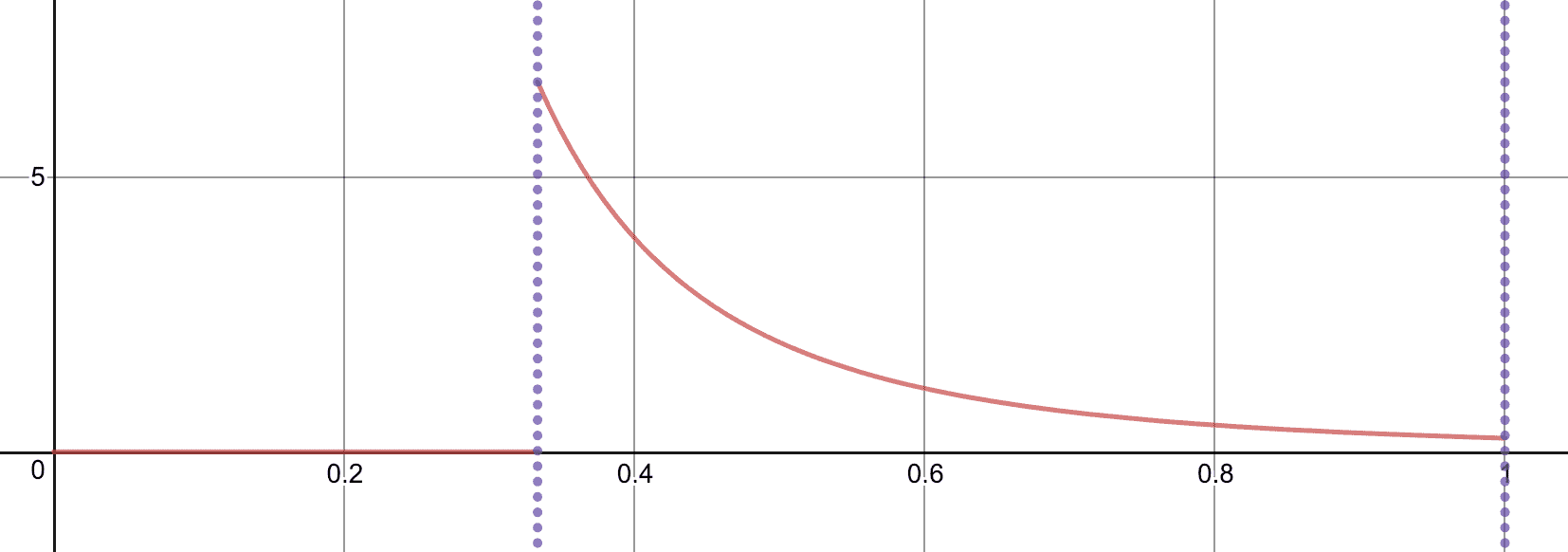
With just one action and P(t) = Q(t) = t, the region before t=1/3 has zero probability, and the probability decreases from 6.75 to 1/4.
Note that the reason $ a_n = 1/3$ is so nice is that $ P(t)$ is so simple. If $ P(t)$ were, say, $ t^2$, then $ a_n$ should shift to being $ \sqrt{1/3}$. If $ P(t)$ were more complicated, we’d have to invert it (or use an approximate search) to find the location $ a_n$ for which $ P(a_n) = 1/3$.
Next, we loosen the example to let $ n=m=4$, still with $ P(t) = Q(t) = t$. In this case, we have the same final interval $ [1/3,1]$. The new actions all occur in the time before $ t=1/3$, in the intervals $ [1/5, 1/3], [1/7, 1/5], [1/9,1/7].$ If there were more actions, we’d get smaller inverse-of-odd-spaced intervals approaching zero. The probability densities are now steeper versions of the same $ 1/4t^3$, with the constant getting smaller to compensate for the fact that $ 1/t^3$ gets larger and maintain the normalized distribution. For example, the earliest interval results in $ \int_{1/9}^{1/7} \frac{1}{16t^3} dt = 1$. Closer to zero the densities are somewhat shallower compared to the size of the interval; for example in $ [1/9, 1/7],$ the density toward the beginning of the interval is only about twice as large as the density toward the end.
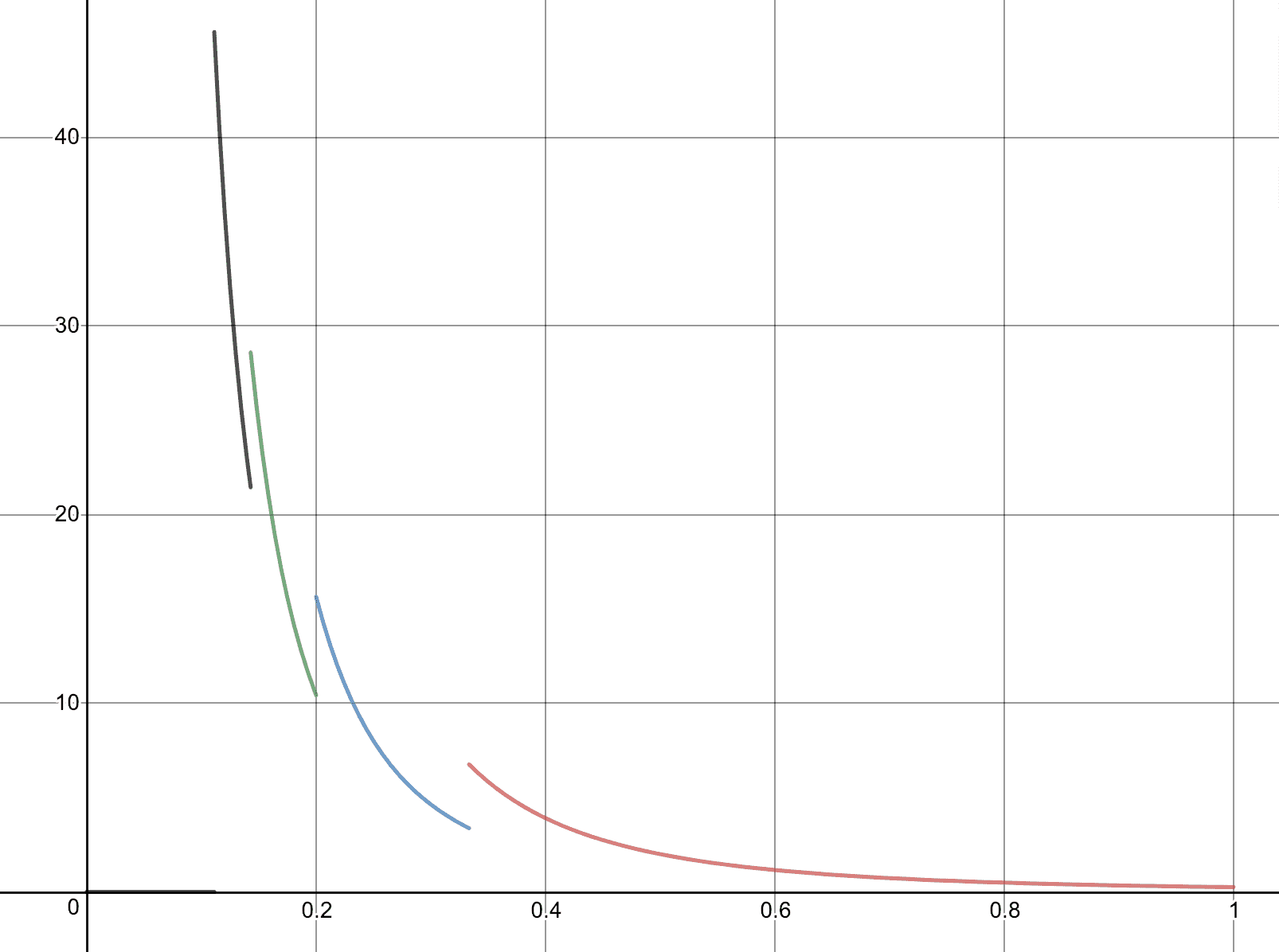
The combination of the four F_i’s for the four intervals in which actions are taken. This is a complete description of the optimal strategy for our simple symmetric version of the silent duel.
Since the early intervals are getting smaller and smaller as we add more actions, the optimal strategy will resemble a burst of action at the beginning, gradually tapering off as the accuracy increases and we work through our budget. This is an explicit tradeoff between the value of winning (lots of early, low probability attempts) and keeping some actions around for the end where you’re likely to succeed.
Next step: get to the example from the general theorem
At this point, we’ve parsed the general statement of the theorem, and while much of it is still mysterious, we extracted some useful qualitative information from the statement, and tinkered with some simple examples.
At this point, I have confidence that the simple symmetric example Restrepo provided is correct; it passed some basic unit tests, like that each $ dF_i$ is normalized. My next task in fully understanding the paper is to be able to derive the symmetric example from the general construction. We’ll do this next time, and include a program that constructs the optimal solution for any input.
Until then!