Graph Coloring, or Proof by Crayon

A common visual aid for maps is to color the regions of the map differently, so that no two regions which share a border also share a color. For example, to the right is a map of the provinces of Costa Rica (where the author is presently spending his vacation). It is colored with eight different colors, one for each province. Of course, before the days of 24-bit “true color,” designing maps was a long and detailed process, and coloring them was expensive. It was in a cartographer’s financial interest to minimize the number of colors used for any given map. This raises the obvious question, what is the minimum number of colors required to color Costa Rica in a way that no two provinces which share a common border share a common color?

With a bit of fiddling, the reader will see that the answer is obviously three. The astute reader will go further to notice that this map contains a “triangle” of three provinces which pairwise share common borders. Hence even these three alone cannot be colored with just two.

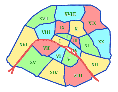
This problem becomes much trickier, and much more interesting to we mathematicians, as the number of provinces increases. So let us consider the map of the arrondissements of Paris.

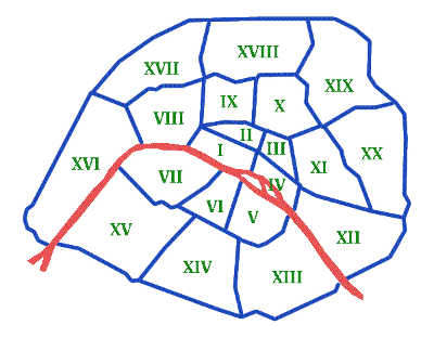
With so many common borders, we require a more mathematically-oriented description of the problem. Enter graph theory.

Let us construct an undirected graph $ P$ (for Paris), in which the vertices are the arrondissements, and two vertices are connected by an edge if and only if they share a common border. In general, when we color graphs we do not consider two regions to share a border if their borders intersect in a single point, as in the four corners of the United States. Performing this construction on Paris, we get the following graph. Recognizing that the positions of the corresponding vertices are irrelevant, we shift them around to have a nicely spread-out picture.

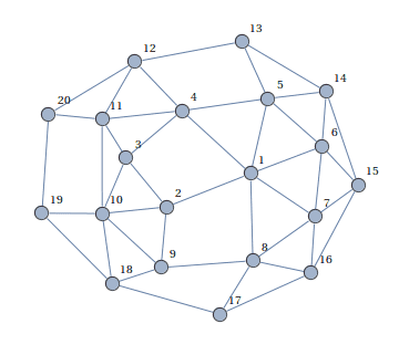
Now that the relationships between arrondissements are decidedly unambiguous, we may rigorously define the problem of coloring a graph.

Definition: A coloring of a graph $ G = (V,E,\varphi )$ is a map $ f: V \to \left \{ 1 \dots n \right \}$, such that if $ v,w \in V$ are connected by an edge, then $ f(v) \neq f(w)$. We call $ n$ the size of a coloring, and if $ G$ has a coloring of size $ n$ we say that $ G$ is $ n$-colorable, or that it has an $ n$-coloring.

Definition: The chromatic number of a graph $ G$, denoted $ \chi(G)$ is the smallest positive number $ k$ such that $ G$ is $ k$-colorable.

Our first map of Costa Rica was 3-colorable, and we saw indeed that $ \chi(G) = 3$.

We now turn our attention to coloring Paris. To do so, we use the following “greedy” algorithm. For the sake of the pseudocode, we represent colors by natural numbers.

Given a set of vertices V of a graph G:
   For each vertex w in V:
      let S_w be the set of colors which have been previously
        assigned to neighbors of w
      Color w with the smallest number that is not in S_w

Obviously, the quality of the coloring depends on the order in which we investigate the vertices. Further, there always exists an ordering of the vertices for which this greedy algorithm produces a coloring which achieves the minimum required number of colors, $ \chi(G)$. Applying this to Pairs, we get the following 4-coloring:

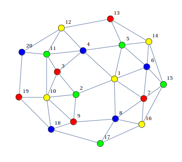
Translating this back into its original form, we now have a pretty picture of Paris.

But this is not enough. Can we do it with just three colors? The call of the wild beckons! We challenge the reader to find a 3-coloring of Paris, or prove its impossibility. In the mean time, we have other matters to attend to.

We note (without proof) that to determine $ \chi(G)$ algorithmically is NP-complete in general. Colloquially this means a fast solution is believed not to exist, and to find one (or prove this belief is true) would immediately make one the most famous mathematician in the world. In other words, it’s very, very hard. The only general solutions take at worst an exponential or factorial amount of time with regards to the number of vertices in the graph. In other words, trying to run a general solution on a graph of 50 vertices is likely to take 50! (a 65-digit number) steps to finish, far beyond the computational capacity of any computer in the foreseeable future.

We Are But Planar Fellows, Sir.

Now we turn to a different aspect of graph theory, which somewhat simplifies the coloring process. The maps we have been investigating thus far are special. Specifically, their representations as graphs admit drawings in which no two edges cross. This is obvious by our construction, but on the other hand we recognize that not all graphs have such representations. For instance, try to draw the following graph so that no two edges cross:

If it seems hard, that’s because it’s impossible. The proof of this fact requires a bit more work, and we point the reader in the direction of Wagner’s Theorem. For now, we simply recognize that not all graphs have such drawings. This calls for a definition!

Definition: A simple graph is planar if it can be embedded in $ \mathbb{R}^2$, or, equivalently, if it can be drawn on a piece of paper in such a way that any two intersecting edges do so only at a vertex.

As we have seen, the graphs corresponding to maps of arrondissements or provinces or states are trivially planar. And after a lifetime of cartography, we might notice that every map we attempt to color admits a 4-coloring. We now have a grand conjecture, that every planar graph is 4-colorable.

The audacity of such a claim! You speak from experience, sir, but experience certainly does not imply proof. If we are to seriously tackle this problem, let us try a simpler statement first: that every planar graph is 5-colorable. In order to do so, we need a few lemmas:

Lemma: If a graph $ G$ has $ e$ edges, then $ \displaystyle 2e = \sum \limits_{v \in V} \textup{deg}(v)$.

Proof. Since the degree of a vertex is just the number of edges touching it, and every edge touches exactly two vertices, by counting up the degrees of each vertex we count twice the number of edges. $ \square$

Lemma: If a planar graph $ G$ has $ e$ edges and $ f$ faces (regions bounded by edges, or the exterior of a graph) then $ 2e \geq 3f$, and $ f \leq (2/3) e$.

Proof. In a planar graph, every face is bounded by at least three edges (by definition), and every edge touches at most two faces. Hence, $ 3f$ counts each edge at most twice, while $ 2e$ counts each face at least three times. $ \square$.

We also recognize without proof the Euler Characteristic Formula for Planar Graphs, (which has an equally easy proof, provided you understand what an edge contraction is): $ n-e+f=2$, where $ G$ has $ n$ vertices, $ e$ edges, and $ f$ faces.

Lemma: Every planar graph has a vertex of degree less than 6.

Proof. Supposing otherwise, we may arrive at a contradiction in Euler’s formula: $ 2 = v – e + f \leq v – e + (2/3) e$, so rearranging terms we get $ e \leq 3v – 6$, and so $ 2e \leq 6v – 12$. Recall that $ 2e$ is the sum of the degrees of the vertices of $ G$. If every vertex has degree at least 6, then $ 6v \leq 2e \leq 6v – 12$, which is just silly. $ \square$.

This is all we need for the five color theorem, so without further ado:

Theorem: Every planar graph admits a 5-coloring.

Proof. Clearly every graph on fewer than 6 vertices has a 5-coloring. We proceed by induction on the number of vertices.

Suppose to the contrary that $ G$ is a graph on $ n$ vertices which requires at least 6 colors. By our lemma above, $ G$ has a vertex $ x$ of degree less than 6. Removing $ x$ from $ G$, the inductive hypothesis provides a 5-coloring of the remaining graph on $ n-1$ vertices. We simply need to color $ x$ with one of these five colors, and the theorem is proved.

If $ x$ has fewer than 5 neighbors or its neighbors use fewer than 5 colors, then we may assign it the color that is not used in any of its neighbors. Otherwise, we may assume $ x$ has five neighbors, and each neighbor has a distinct color (presumably requiring $ x$ to have the sixth, new color). Let $ v_1, v_2, v_3, v_4, v_5$ be the neighbors of $ x$, labelled in some clockwise order around $ x$, and say they have colors $ 1,2,3,4,5$, respectively.

Consider $ G_{1,3}$, the subgraph of $ G$ which contains only vertices of colors 1 and 3. There are two cases: either $ v_1$ is in the same connected component as $ v_3$ (there exists a path connecting them which does not go through $ x$), or not. If not, then we may take the component which contains $ v_1$, and switch the colors 1 and 3. Then $ x$ is connected to two vertices of color 3, and we may color it 1.

Otherwise, there is a path from $ v_1$ to $ v_3$. This path is special, because with $ x$, the path $ v_1 v_3 x$ completely encapsulates $ v_2$ with vertices of colors 1 and 3 (and $ x$). The planarity of the graph implies, then, that $ v_2$ cannot be connected to either of $ v_4$ or $ v_5$. Hence, we may repeat the color-swapping argument on $ G_{2,4}$, the subgraph of colors 2 and 4, to give $ x$ color 2. $ \square$.

So that was entirely done with elementary arguments, and is a pretty neat proof. Of course, we really want the head of the four-color theorem on a mantle, but he is a much more elusive beast.

Computers Doing Proofs? Blasphemy.

But that is what it took to finish off the four-color theorem. Despite a hundred years of research and diversions, it took a brute-force computer search of 1,936 configurations, and over 1200 computer hours, to prove that no counterexample to the four-color theorem exists.

It was proved in 1976 by Appel and Haken, and it was very controversial for a long time, in principle because no human could verify that the computer hadn’t made an error. On the other hand, it was not hard to verify the correctness of the program itself, but after 1200 CPU hours, who can guarantee a bit wasn’t mistakenly flipped by some cosmic rays or a magnetic malfunction? Luckily, the proof was further simplified and reproved over the next twenty years, so today the problem is widely believed to be solved.

So indeed it is true! We may color every map with just four colors! Unfortunately, even a sketch of the proof is far beyond the scope of this blog. We are content to marvel at the work ethic of other mathematicians.

Next time, we will discuss the applications of graph coloring to computer problems, such as job scheduling and register allocation in compilers.

Until then!