This post assumes familiarity with the terminology and notation of linear algebra, particularly inner product spaces. Fortunately, we have both a beginner’s primer on linear algebra and a follow-up primer on inner products.

The Quest

We are on a quest to write a program which recognizes images of faces. The general algorithm should be as follows.

1. Get a bunch of sample images of people we want to recognize.
2. Train our recognition algorithm on those samples.
3. Classify new images of people from the sample images.

We will eventually end up with a mathematical object called an eigenface. In short, an eigenface measures variability within a set of images, and we will use them to classify new faces in terms of the ones we’ve already seen. But before we get there, let us investigate the different mathematical representations of images.

God has given you one face, and you make yourself a vector

Most naturally, we think of an image as a matrix of pixel values. For simplicity, we restrict our attention to grayscale images. Recall that a pixel value in the standard grayscale model is simply an unsigned byte representing pixel intensity. In other words, each pixel is an integer ranging from 0 to 255, where 0 is black and 255 is white. So every $ n \times m$ image corresponds bijectively to a matrix with integer entries between 0 and 255.

Representing an image as a matrix reminds us of the ubiquitous applicability of linear algebra. Indeed, we may learn a great deal about our image by representing it with different bases or querying pixel neighbors. We can find frequencies, detect edges, and do a whole host of other fascinating things. However, we aren’t only concerned with the properties of one picture. In fact, individual pictures are useless to us! We only care about the relationships between a set of pictures, and we want to be able to compute “how similar” two faces are to each other.

In other words, we want a face space.

So instead of representing our images as a matrix, let’s represent them as points. Given an $ n \times m$ matrix $ A$ with entries $ a_{i,j}$, we simply “collapse” the rows of a matrix into a single row like so:

$ v = (a_{1,1}, \dots , a_{1,m}, a_{2,1}, \dots , a_{2,m}, \dots , a_{n,1}, \dots , a_{n,m})$

Now we have our face space: $ \mathbb{R}^{n m}$. Note that even for small images, this space is huge. For example, with images of size $ 100 \times 100$, this space has ten-thousand dimensions! Certainly, reasoning about such objects would be impossible without a computer, but even then, we will run into trouble.

In order to translate back and forth between the standard matrix representation and the vector representation, we present the following Mathematica code. As always, the full notebook including all the code we provide here is available on this blog’s Github page.

imageToVector[img_] := Flatten[ImageData[img]];
vectorToImage[vec_, {n_, m_}] := Image[Partition[vec, m]];

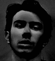
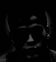
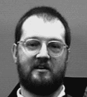
Now all we need is a set of example faces. We found such an example from a facial recognition research group, and we posted the images on our Google code page. It contains a large number of images of size $ 200 \times 180$ pixels. Here are a few samples:

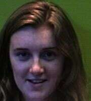
This bounty of data is excellent. Now we may begin to play.

Mean Faces

In order to classify faces we would like to investigate the distribution of faces in face space. We start by computing the “mean face,” which represents the center of gravity of our sample of faces. We can do this simply by averaging the values of each pixel across all our face images.

We start by selecting a sample of male faces, at most one for each person in our database, and transforming them to grayscale:

(* This directory is particular to my file system. Change it
appropriately. *)

files = Import["~/downloads/faces94/male"][[1 ;; -1 ;; 30]];
faces = Map[Import["~/downloads/faces94/male/" <> #] &, files];

grayFaces = Map[ColorConvert[#, "Grayscale"] &, faces];

Then, we construct a vector with the average pixel intensity values for each pixel:

meanImage = Image[
  Apply[Plus, Map[ImageData, grayFaces]] / Length[grayFaces]
]

ImageData accepts an image object (as represented in Mathematica) and returns the matrix of pixel values. Note that for this particular operation, which is just adding and dividing, it is unnecessary to translate faces from matrices to vectors.

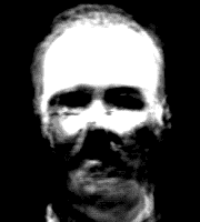
The result is the following image:

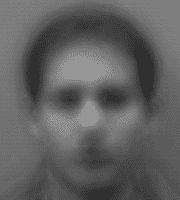
Honestly, for a mean face I expected something more sinister. Just for kicks, let’s watch the averaging process incrementally:

This is a nice (seemingly fast) convergence. We casually wonder how much this particular image is subject to change with data coming from different cultures, as most of our data are twenty- or thirty-something white males.

Now that we have a mean, we may calculate the deviations of each image from our mean. Again, this is a simple subtraction of pixel values, which does not require special representation.

differenceFaces = Map[ImageSubtract[#, meanImage]&, grayFaces];

And get some pictures that look like these:

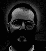
Don’t they look much nicer now that we’ve subtracted off the mean face? In all seriousness, we call these difference faces.

As one can see, some of these difference faces are darker than others. For whatever reason (perhaps some faces are in slightly more agreeable positions), the lighter faces are more “unique” in this sample of faces. We will see this notion come up again when we compute the actual eigenfaces: some will resemble the more variable faces.

While this is fine and dandy, we don’t yet have a way to recognize anybody. For this, we turn to statistics.

Covariance

We may interpret our face vectors in face space as a distribution of $ n$ random variables which are precisely the people in the training sample. Specifically, when we try to classify a new face, we want to calculate the distance of that face from each of our training faces, and infer how likely it is to be a specific person.

In reality, however, since our faces are points in a space of $ 180 \times 200 = 36,000$ dimensions, we have $ 36,000$ random variables: one for each coordinate axis. While we recognize that this is far too many variables for us to do any computations with, we play along for now.

Taking our cue from statistics, we want to investigate the variability of the set of face vectors. To do this we use a special matrix called the covariance matrix of our distribution.

Definition: The covariance of two variables, denoted $ \textup{Cov}(x,y)$, is the expected value of the product of their deviations from their means: $ \textup{E}[(x-\textup{E}[x])(y-\textup{E}[y])]$.

Colloquially, the covariance measures the relationship between how two variables change. A high positive covariance means that a positive change in one variable correlates to a positive change in the other. A highly negative covariance implies a positive change in one variable correlates to a negative change in the other. If the two variables are independent, then their covariance is zero, though the reverse implication is not true in general.

As an example, consider the following distribution of points in the plane:

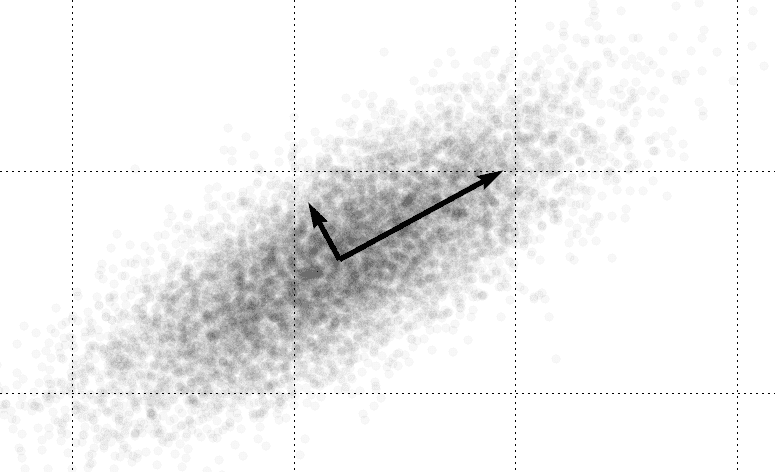
This distribution clearly has a nontrivial covariance in the $ x$ and $ y$ variables. It looks like an ellipse on a tilted axis signified by the two black arrows. In fact, we will soon be able to calculate those arrows; they have very special significance for us.

So just finding the variance of $ x$ and $ y$ (as in the coordinate axes) is not enough to fully describe this distribution. We need three numbers: the variance of $ x$, the variance of $ y$, and the covariance of $ x,y$. As a side note, the variance of a variable is equivalently the covariance of that variable with itself.

We represent these three pieces of data in a covariance matrix, which for the two variables above has the form:

$ \begin{pmatrix} \textup{Cov}(x,x) & \textup{Cov}(x,y) \\ \textup{Cov}(y,x) & \textup{Cov}(y,y) \end{pmatrix}$

Since the “Cov” as a function is symmetric in its arguments, we see that every covariance matrix is symmetric. This will have important implications for us, as symmetric matrices have a rich theory for us to exploit.

Once we compute the covariance matrix of our two variables, we want to describe the variance in terms of the “axes” as above. In other words, if we could just tilt, stretch, and move the data the right way, we could put it back on top of the normal unit coordinate axes $ (1,0)$ and $ (0,1)$. The process we just described is precisely a linear map that performs a change of basis. In particular, those two black arrows constitute the best basis to describe the data. So if we could just compute the right basis, we’d know everything about our distribution!

Now it’s no coincidence that the particular basis above is so nice. Specifically, if we consider our random variables as unit measurements along those axes (remember, one axis is stretched, so a unit measurement is longer there), then the two variables have zero covariance. In particular, the covariance matrix of the random variables in that basis is diagonal! Recalling that if a matrix has a diagonal representation, then the basis for that representation is a basis of eigenvectors. Hence, we see that computing any basis of eigenvectors will give us our optimal basis, should one exist.

And now, the coup de grâce, we recall that every symmetric real-valued matrix, and hence every covariance matrix, has an orthonormal basis of eigenvectors! This is a special case of the spectral theorem, which we discuss in our primer on inner product spaces.

So now we have proven that for any distribution of data in $ n$ random variables, we may describe them with a basis of eigenvectors, such that the variables are pairwise uncorrelated. Let’s apply this to our face space.

Methinks no eigenface so gracious is as mine

In one mindset, we may compute the covariance matrix of our difference faces quite easily:

differenceVectors = Map[imageToVector, differenceFaces];
covarianceMatrix = Transpose[differenceVectors].differenceVectors;

For the Java coders, note that the dot notation is for vector products; Mathematica is not object oriented, but rather it is functional with built in hash maps for mutation. Furthermore, in it’s raw form the “differenceVectors” variable is a 76-element list of face vectors.

These dot products, however, are precisely the computations of covariance, since each dot product computed is between two difference face vectors, each component of which is one of our random variables. Perform a few of the computations by hand (on a smaller matrix, obviously!) to convince yourself that it is so. The $ i,j$ entry of our resulting covariance matrix is just $ \textup{Cov}(x_i,x_j)$.

Here we are multiplying a $ 36,000 \times 76$ matrix (76 face vectors of length 36,000) by a $ 76 \times 36,000$ matrix, resulting an a $ 36,000 \times 36,000$ matrix. While we could theoretically compute the eigenvalues and eigenvectors of this matrix directly, in reality even the matrix multiplication to construct the matrix uses up all available memory and crashes the Mathematica kernel (how wimpy my netbook is that it can’t handle a billion-entry matrix!). In any case, we need another way to get our eigenvectors.

Again going back to linear algebra, we have a few useful propositions:

Proposition: If $ A$ is a real matrix, then $ AA^{\textup{T}}$ and $ A^{\textup{T}}A$ are symmetric square matrices.

Proof. The squareness of these products is trivial. We prove symmetry of the first, and note the argument is identical for the second.

Here symmetry is equivalent to $ A^{\textup{T}}A = (A^{\textup{T}}A)^{\textup{T}}$. We can see this immediately by using properties of transposition. Alternatively, we can note that the $ i,j$ entry of the left side is the dot product of the $ i$th row of $ A^{\textup{T}}$ with the $ j$th row of $ A$. On the other hand, the $ j,i$ entry is the dot product of the $ j$th column of $ A^{\textup{T}}$ and the $ i$th column of $ A$. Since the two factors are transposes of each other, the $ i$th row of $ A^{\textup{T}}$ is equal to the $ i$th column of $ A$, and similarly for the $ j$s. In other words, the dot products described for the $ i,j$ and $ j,i$ entries are dot products of the same two vectors, and are hence equal. $ \square$

In particular, we will use the symmetry about the smaller $ AA^{\textup{T}}$ to get information about the eigenvectors of the larger $ A^{\textup{T}}A$. We just need the following proposition:

Proposition: Let a real matrix $ A$ have dimension $ n \times m$, where $ n \leq m$ (here a transposition of $ A$ maintains generality). Then the number of eigenvectors with nonzero eigenvalue of $ A^{\textup{T}}A \ (m \times m)$ is no greater than the number of eigenvectors with nonzero eigenvalue of $ AA^{\textup{T}} \ (n \times n)$

In particular, the eigenvectors with zero eigenvalues are removable; they correspond to zero variability of a face in that particular direction. So for our purposes, it suffices to find the eigenvalues with nonzero eigenvalue. As we are about to see, this is generally much smaller than the total number of eigenvectors. In fact, the result above follows from a stronger statement:

Proposition: If $ v$ is an eigenvector with nonzero eigenvalue of $ A^{\textup{T}}A$, then $ Av$ is an eigenvector with the same eigenvalue of $ AA^{\textup{T}}$.

Proof. Letting $ v$ be such an eigenvector, with corresponding eigenvalue $ \lambda \neq 0$, we have $ A^{\textup{T}}Av = \lambda v$, and hence

$ (AA^{\textup{T}})Av = A(A^{\textup{T}}A)v = A \lambda v = \lambda Av$

This completes the proof. $ \square$

By the same reasoning, if $ v$ is an eigenvector with nonzero eigenvalue of $ AA^{\textup{T}}$, then $ A^{\textup{T}}v$ is an eigenvector of $ A^{\textup{T}}A$.

Now we have just given a bijection between the eigenvectors with nonzero eigenvalue of $ AA^{\textup{T}}$ and the much smaller $ A^{\textup{T}}A$! This is great, because if we compute in our face problem, the former is a mere $ 76 \times 76$ matrix! Computing the eigenvectors is then a one-line affair, utilizing Mathematica’s fast library for it:

eigenfaceSystem = Eigensystem[covarianceMatrix];

This returns the eigenvalues in decreasing order, with their corresponding eigenvectors attached. Note that we still need to multiply them by the transpose of our “differenceVector” matrix.

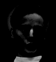
The astute reader will notice that we named these eigenvectors eigenfaces. Though they are indeed just plain old eigenvectors, they have a special interpretation as images. Reforming them as $ 200 \times 180$ grayscale pictures, and scaling the values to $ [0,255]$, we reveal truly haunting faces:

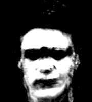
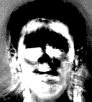
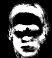
As creepy as they look, one must recall their astonishing interpretation: each ghostly face represents a random variable and the largest change of that random variable along its axis. Specifically, by finding these eigenfaces, we translated our notion of dimension from having one for each pixel to having one for each person in our training set, and these eigenfaces represent shared variability among the faces of those people. In other words, these faces represent the largest similarities between some faces, and the most drastic differences between others. This is one of the most stunning visualizations of dimension this mathematician has ever seen.

This Face is Your Face, This Face is My Face

Though we only display a few above, we computed a basis of 76 different eigenfaces. Call the subspace spanned by these basis vectors (which is certainly a small subspace of $ \mathbb{R}^{36,000}$) the eigenface subspace. For the purpose of learning new faces, we may reduce face space to the eigenface subspace, and hence represent any face as a linear combination of the eigenfaces.

To do this, we recall once again that the spectral theorem not only provided us a basis of eigenvectors, but it guaranteed that this basis is orthonormal. Recalling our primer, the projections of a vector onto elements of an orthonormal basis give us the needed coefficients for that vector’s expansion. If we label our eigenfaces $ f_i$, then any face $ c$ can be decomposed as

$ c = \left \langle c, f_1 \right \rangle f_1 + \dots + \left \langle c,f_{76} \right \rangle f_{76}$

Here since we are working within $ \mathbb{R}^{36,000}$, we may simply use the standard dot product as our inner product. Hence, in Mathematica the coefficients are easy to compute:

projectImageToFaceSpace[image_, meanImage_, eigenfaces_]:=
 Module[{imageVec, diffVec, meanVec},
  imageVec = imageToVector[image];
  meanVec = imageToVector[meanImage];
  diffVec = imageVec - meanVec;
  Map[(diffVec.#)&, eigenfaces]
 ];

For the following face, we present its coefficients when projected onto each of the 76 eigenfaces, in order by decreasing eigenvalues.

coefficients =
 {-6.85693, 23.7498, -11.4515, -3.43352, 5.24749, -7.1615,
  8.09015, -9.7205, -0.660834, -2.4148, -10.3942, 3.33424,
  2.94988, -2.75981, 3.02687, -2.4499, -2.09885, -5.98832,
  -4.22564, -0.65014, 2.20144, -5.43782, -9.61821, -3.25227,
  7.49413, -0.145002, 7.61483, -0.696994, -3.7731, 3.23569,
  -1.78853, 0.0400116, -3.86804, -2.02456, 2.20949, -1.86902,
  1.23445, 0.140996, 0.698304, -0.420466, 2.30691, 3.70434,
  1.02417, 0.382809, 0.413049, -0.994902, 0.754145, 0.363418,
  -0.383865, 1.46379, 1.96381, -2.90388, -2.33381, -0.438939,
  -0.30523, -0.105925, 0.665962, -0.729409, -1.28977, 0.150497,
  0.645343, 0.30724, -1.04942, 1.0462, -0.60808, 0.333288,
  1.09659, -1.38876, 0.33875, 0.278604, 1.0632, -0.0446148,
  0.24526, -0.283482, -0.236843, 0.312122};

And with the following piece of code, we can reconstruct the image exactly from the eigenfaces:

vectorToImage[
  imageToVector[meanImage] + Apply[Plus, coefficients*eigenfaces],
{200, 180}]

While this is fine and dandy, we can do better computationally. As the magnitude of an eigenface’s corresponding eigenvalue decreases, we see, both visually and mathematically, that the eigenface contributes less to the overall variability of the distribution of faces. In other words, we can shed some of the shorter coordinate axes and still retain most of our description of face space!

Here is an animation of the face reconstruction where we choose the first $ k$ eigenfaces (i.e., with the largest $ k$ corresponding eigenvalues), and increase $ k$:

We notice some “pauses” in the animation, which correspond to either very small coefficients or eigenfaces which only have small regions of variability.

Unfortunately, and this is in the author’s opinion an inherent wishy-washiness of applied mathematics, how many eigenfaces to use is an empirically determined variable. Exercising our best judgement, we find that the image reconstruction is easily recognizable after 30 eigenfaces are used (about seven seconds into the animation above), so we use those for our reduced eigenface subspace.

Recognition Procedure

Now, to polish off our discussion, we have the quite simple recognition procedure. Once we have projected every sample image into the eigenface subspace, we have a bunch of points in $ \mathbb{R}^{76}$.

When given a new image, all we need do is project it into face space, and find the smallest distance between the new point and each of the projections of the sample images. We do so in the Mathematica notebook (available from this blog’s Github page), and also run the recognition procedure on some pictures of the training subjects not used in training.

The reader is invited to look at the results, and see what sorts of changes in appearance mess up recognition the most. As a sneak preview, it seems that head-tilting, eye-closing, and smiling account for a lot of variability. If the reader is a fugitive on the run (and somehow find’s time to read this blog; I’m so honored!), and wishes to have his photograph not recognized, he should smile, tilt his head, and blink vigorously while the photograph is being taken. Additionally, to avoid detection, he should split some of his heist money with the author.

We notice one additional problem: in our haphazard way of selecting individuals for training and evaluation, we mistakenly attempted to classify some individuals that were never in a training photo. What’s worse, is that some of these men look strikingly similar to different people who were used in the training photos, with obvious differences like ears which stick out or thicker noses.

To handle subjects who were not in training, we need a category for those individuals who could not be classified. This is straightforward enough; we just have a minimum threshold. If an image is not within, say 25 units of any of our training faces, then it cannot be classified. This threshold can only be chosen empirically, which is again an unfortunate consequence of moving from pure mathematics to the real world.

With this modification, we see that our final evaluation sample of thirty faces, three of which were not in the original training set, results in only two false positive matches, and one false negative. This method appear to be relatively robust, considering its simplicity.

For more precise results, the reader is encouraged to play with the data and run larger tests. The faces used are organized by gender and name in a downloadable zip file on this blog’s Github page. The archive contains about twenty photos for each individual, and about eighty individuals. Have a blast!

An Alternative Metric

While Euclidean distance is fine and dandy, there are a whole host of other methods for classifying points in Euclidean space. One could potentially train a neural network to perform classification, or dig deeper down the linear algebra rabbit hole and run the points through a support vector machine. Of course, with the rich ocean of literature on classification problems, there are likely many other applicable methods that the reader could explore. [Note: we intend to cover both neural networks and support vector machines on this blog in due time.]

However, there is one less drastic change we can make in our recognition procedure: ditch Euclidean distance. We may want to do so because our axes (the eigenfaces, which recall are eigenvectors of random variables), are at different scales. Euclidean distance hence treats one unit along a short axis as importantly as it treats a fraction of a longer axis. But the distances along shorter axes are more variable, and hence a small change there should mean more than it does elsewhere. This simply cannot do.

Our remedy is the Mahalanobis metric. It is specifically designed to utilize the covariance matrix to measure weighted distances.

Definition: Given a covariance matrix $ S$, the Mahalanobis metric $ m$ is defined as

$ \displaystyle m(x,y) = \sqrt{(x-y)^{\textup{T}} S^{-1} (x-y) }$

However, since our covariance matrix is diagonal (using our basis of eigenvectors, the entries are just the corresponding eigenvalues), $ S^{-1}$ is easy to compute: we just invert each diagonal entry. We encourage the reader to compare the two distance metrics’ performance in eigenface recognition. Augmenting our Mathematica notebook to do so should not require more than a few lines of code.

Finally, a few extensions and modifications of the eigenface method have popped up since their conception in the late 1980’s. In particular, they seek to compensate for the eigenface approach’s weakness to changes in lighting, orientation, and scaling. One such method is called “fisherfaces,” another “eigenfeatures,” and yet another the “active appearance model.” The latter two appear to map out “landmarks” on the image being processed, combining traditional facial metrics or anomalies with the eigenface decomposition technique. This author may return to an investigation of other facial recognition systems in the future, but for now we have too many other ideas.

Additional Uses

The eigenface method for facial recognition hints at a far more general technique in mathematics: breaking an object down into components which yield information about the whole. This is everywhere in mathematics: group theory, Fourier analysis, and of course linear algebra, to name a few. For linear algebra, the method is called principal component analysis, and this method has wide application in both statistics and machine learning methods in general (which are nowadays largely statistical procedures anyway).

Aside from using eigenfaces to classify faces or other objects, they could be used simply for facial detection. The projection of a facial image into face space, whether the image is used for training or not, will almost always be relatively close to some training image. While the distance might not be small enough to determine a person’s identity, it is usually close enough to determine whether the image is of a face. We encourage the reader to use our code to write a function for facial detection. We anticipate it require less than twenty lines of code, and it should be very similar to our function for classification.

Another simplified application is to classify gender. We casually wonder if it would be more robust, and point the reader to this paper on it. The researcher here has a shockingly high-quality data set, and he also tries his hand on some general, low-quality data sets. It’s a good, quick read for one who has absorbed the content here.

Finally, eigenfaces can also be used as a method for image compression. Since we reduce an image to the 76 coefficients used to rebuild it from the eigenfaces, we see that an image is compressed from being 36,000 bytes to 76 floats. With a large collection of thousands of images and an agreeable tolerance for image approximation, eigenfaces could save quite a lot of space.

So we see that even though our original task was to classify faces, we have stumbled upon a whole host of other solutions to problems in computer science. Indeed, a method for image compression is quite far from the pure mathematics of orthonormal eigenvector bases. We attribute the connections to the beauty of mathematics and computer science, and look forward to the next time we may witness such a connection.

Until then!