This post assumes some basic familiarity with Euclidean geometry and linear algebra. Though we do not assume so much knowledge as is contained in our primer on inner product spaces, we will be working with the real Euclidean inner product. For the purpose of this post, it suffices to know about the “dot product” of two vectors.
The General Problem
One of the main problems in machine learning is to classify data. Rigorously, we have a set of points called a training set $ X = \left \{ \mathbf{p_i} \right \} \subset \mathbb{R}^n$ generated by some unknown distribution $ D$. These points are often numerical representations of real-world data. For instance, one dimension could represent age, while another could represent cholesterol level. Then each point $ \mathbf{p_i}$ would be a tuple containing the relevant numerical data for a patient. Additionally, each point has an associated label $ l_i = \pm 1$, which represents the class that piece of data belongs to. Continuing our cholesterol example, the labels here could represent whether the patient has heart disease. For now, we stick to two classes, though iterated techniques extend any binary classification method to a multiple-class problem.
Given such a training set, we seek a decision function $ f : \mathbb{R}^n \to \left \{ \pm 1 \right \}$ which is consistent with our training set (i.e. $ f(\mathbf{p_i}) = l_i$ for each $ i$) and generalizes well to all data generated by $ D$ (i.e. new data points not part of the training set). We want our decision function to treat future heart-disease patients as well as correctly classify those from the past.
With no restrictions on $ f$, one would imagine such a function is wild! In fact, if the distribution $ D$ has no patterns in it (e.g. random noise), then no such $ f$ exists. However, for many distributions one can discover functions which are good approximations. They don’t even have to be consistent with the training set, as long as they work reliably in general.
Arguably the simplest non-trivial example of such a decision function is a line in the plane which separates a training set $ X \subset \mathbb{R}^2$ into two pieces, one for each class label. This is precisely what the perceptron model does, and it generalizes to separating hyperplanes in $ \mathbb{R}^n$.
The Dawn of Machine-Kind: the Perceptron
The very first algorithm for classification was invented in 1957 by Frank Rosenblatt, and is called the perceptron. The perceptron is a type of artificial neural network, which is a mathematical object argued to be a simplification of the human brain. While at first the model was imagined to have powerful capabilities, after some scrutiny it has been proven to be rather weak by itself. We will formulate it in its entirety here.
Most readers will be familiar with the equation of a line. For instance, $ y = -2x$ is a popular line. We rewrite this in an interesting way that generalizes to higher dimensions.
First, rewrite the equation in normal form: $ 2x + y = 0$. Then, we notice that the coefficients of the two variables form a vector $ (2,1)$, so we may rewrite it with linear algebra as $ \left \langle (2,1),(x,y) \right \rangle = 0$, where the angle bracket notation represents the standard Euclidean inner product, also known as the dot product. We note that by manipulating the values of the coefficient vector, we can get all possible lines that pass through the origin.
We may extend this to all lines that pass through any point by introducing a bias weight, which is a constant term added on which shifts the line. In this case, we might use $ -1$ to get $ \left \langle (1,2),(x,y) \right \rangle – 1 = 0$. The term “bias” is standard in the neural network literature. It might be better to simply call it the “constant weight,” but alas, we will follow the crowd.
We give the coefficient vector and the bias special variable names, $ \mathbf{w}$ (for the common alternative name weight vector) and $ b$, respectively. Finally, the vector of variables $ (x,y)$ will be henceforth denoted $ \mathbf{x} = (x_1, x_2, \dots , x_n)$. With these new naming conventions, we rewrite the line equation (one final time) as $ \left \langle \mathbf{w}, \mathbf{x} \right \rangle + b = 0$.
Now we let the dimension of $ \mathbb{R}^n$ vary. In three dimensions, our $ \left \langle \mathbf{w}, \mathbf{x} \right \rangle + b = 0$ becomes $ w_1x_1 + w_2x_2 + w_3x_3 + b = 0$, the equation of a plane. As $ n$ increases, the number of variables does as well, making our “line” equation generalize to a hyperplane, which in the parlance of geometry is just an affine subspace of dimension $ n-1$. In any case, it suffices to picture a line in the plane, or a plane in three dimensions; the computations there are identical to an arbitrary $ \mathbb{R}^n$.
The usefulness of this rewritten form is in its evaluation of points not on the hyperplane. In particular, we define $ f : \mathbb{R}^n \to \mathbb{R}$ by $ f(\mathbf{x}) = \left \langle \mathbf{w}, \mathbf{x} \right \rangle + b$. Then taking two points $ \mathbf{x,y}$ on opposite sides of the hyperplane, we get that $ f(\mathbf{x}) < 0 < f(\mathbf{y})$ or $ f(\mathbf{y}) < 0 < f(\mathbf{x})$.
So if we can find the right coefficient vector and bias weight, such that the resulting hyperplane separates the points in our training set, then our decision function could just be which side of the line they fall on, i.e. $ \textup{sign}(f(\mathbf{x}))$. For instance, here is a bunch of randomly generated data in the unit square in $ \mathbb{R}^2$, and a separating hyperplane (here, a line).

The blue region is the region within the unit square where $ f(\mathbf{x}) \geq 0$, and so it includes the decision boundary. If we receive any new points, we could easily classify them by which side of this hyperplane they fall on.
Before we stop to think about whether such a hyperplane exists for every data set (dun dun dun!) let’s go ahead and construct an algorithm to find it. There is a very straightforward way to proceed: as long as the separating hyperplane makes mistakes, update the coefficient vector and bias to remove a mistake. In order to converge, we simply need that the amount by which we push the coefficient vector is small enough. Here’s a bit of pseudocode implementing that idea:
hyperplane = [0, 0, ..., 0], bias = 0
while some misclassification is made in the training set:
   for each training example (point, label):
      if label * (<hyperplane, point> + bias) <= 0:
         hyperplane += label * point
         bias += label
Upon encountering an error, we simply push the coefficients and bias in the direction of the failing point. Of course, the convergence of such an algorithm must be proven, but it is beyond the scope of this post to do so. The interested reader should see these “do-it-yourself” notes. The proof basically boils down to shuffling around inequalities, squeezing things, and applying the Cauchy-Schwarz inequality. The result is that the number of mistakes made by the algorithm before it converges is directly proportional to the volume enclosed by the training examples, and inversely proportional to the smallest distance from the separating hyperplane to any training point.
Implementation (and Pictures!)
As usual, we implemented this algorithm in Mathematica. And albeit with a number of helper functions for managing training sets in a readable way, and a translation of the pseudocode algorithm into functional programming, the core of the implementation is about as many lines as the pseudocode above. Of course, we include the entire notebook on this blog’s Github page. Here are our results:
We generate a set of 25 data points in the unit square, with points above the line $ y = 1-x$ in one class, and those below in the other. This animation shows the updates to the hyperplane at every step of the inner loop, stopping when it finds a separating line.
First, we note that this algorithm does not find “the best” separating line by any means. By “the best,” consider the following three pictures:
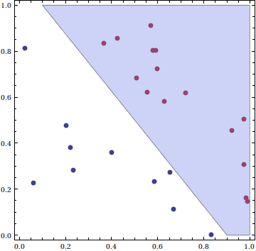
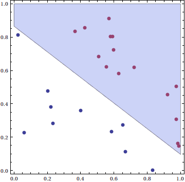
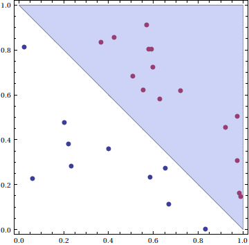
Clearly, the third picture achieves the “best” separation, because it has a larger distance from the training points than the other two. In other words, if we compute the training set margin $ \gamma = \textup{min}(f(\mathbf{p_i}))$, we claim a large $ \gamma$ implies a better separation. While the original perceptron algorithm presented here does not achieve a particularly small $ \gamma$ in general, we will soon (in a future post) modify it to always achieve the maximum margin among all separating hyperplanes. This will turn out to take a bit more work, because it becomes a convex quadratic optimization problem. In other words, finding the best separating hyperplane is conceptually and computationally more difficult than finding any separating hyperplane.
Finally, we test its generalization on a new set of 1000 generated points. We see that even with as few as 25 training samples, we get an accuracy of about 92 percent!
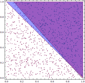
Here the blue region is the region of generated data in class +1, the red region (small sliver in the lower right corner) is the region that the perceptron falsely claims is in class +1, while the purple area is the overlap of the perceptron’s perceived +1 region and the true +1 region.
For a few measly lines of pseudocode, this algorithm packs a punch!
The Problem With Lines
As eagerly as we’d like to apply the perceptron algorithm to solve the problems of the world, we must take a step back and analyze the acceptable problems. In particular (and though this sounds obvious), the perceptron can only find hyperplanes separating things which can be separated by hyperplanes! We call such a training set linearly separable, and we admit that not every training set is so.
The smallest possible such example is three points on a line, where one point in class +1 separates two points in class -1. Historically, however, the first confounding counterexample presented was exclusive “or” function. Specifically, we have four points of the unit square arranged as follows:
(0,0), (1,1) -> +1
(1,0), (0,1) -> -1
The reader can verify that the perceptron loops infinitely on either of the given training sets, oscillating between the same hyperplanes over and over again.
Even though we may not have a linearly separable training set, we could still approximate a separation boundary with a hyperplane. Thus, we’d want to minimize the number of misclassifications of a hyperplane with respect to that training set. Amazingly, this problem in NP-complete. In other words, it is widely believed that the problem can’t be solved in polynomial time, so we can forget about finding a useful algorithm that works on large data sets. For a more complete discussion of NP-completeness, see this blog’s primer on the subject.
The need for linearly separable training data sets is a crippling problem for the perceptron. Most real-world distributions tend to be non-linear, and so anything which cannot deal with them is effectively a mathematical curiosity. In fact, for about twenty years after this flaw was discovered, the world lost interest in neural networks entirely. In our future posts, we will investigate the various ways researchers overcame this. But for now, we look at alternate forms of the perceptron algorithm.
The Dual Representation
We first note that the initial coefficient vector and bias weight for the perceptron were zero. At each step, we added or subtracted the training points to the coefficient vector. In particular, our final coefficient vector was simply a linear combination of the training points:
$$\displaystyle \mathbf{w} = \sum \limits_{i=1}^k \alpha_i l_i \mathbf{p_i}$$Here the $ \alpha_i$ are directly proportional (in general) to the number of times $ \mathbf{p_i}$ was misclassified by the algorithm. In other words, points which cause fewer mistakes, or those which are “easy” to classify, have smaller $ \alpha_i$. Yet another view is that the points with higher $ \alpha_i$ have greater information content; we can learn more about our distribution by studying them.
We may think of the $ \mathbf{\alpha}$ vector as a dual system of coordinates by which we may represent our hyperplane. Instead of this vector having the dimension of the Euclidean space we’re working in, it has dimension equal to the number of training examples. For problems in very high dimension (or perhaps infinite dimensions), this shift in perspective is the only way one can make any computational progress. Indeed, the dual problem is the crux of such methods like the so-called support vector machines.
Furthermore, once we realize that the hyperplane’s coordinate vector can be written in terms of the training points, we may rewrite our decision function as follows:
$$\displaystyle f(\mathbf{x}) = \textup{sign} \left ( \left \langle \sum \limits_{i=1}^k \alpha_i l_i \mathbf{p_i}, \mathbf{x} \right \rangle + b \right )$$By the linearity of an inner product, this becomes
$$\displaystyle f(\mathbf{x}) = \textup{sign} \left ( \sum \limits_{i=1}^k \alpha_i l_i \left \langle \mathbf{p_i}, \mathbf{x} \right \rangle + b \right )$$And the perceptron algorithm follows suit:
alpha = [0, 0, ..., 0], b = 0
while some misclassification is made in the training set:
   for each training example (i, point, label):
      if f(point, label) <= 0:
         alpha[i] += 1
         b += label
So in addition to finding a separating hyperplane (should one exist), we have a method for describing information content. Since we did not implement this particular version of the perceptron algorithm in our Mathematica notebook, we challenge the reader to do so. Once again, the code is available on this blog’s Github page, and feel free to leave a comment with your implementation.
Until next time!
Want to respond? Send me an email, post a webmention, or find me elsewhere on the internet.