And a Pinch of Python
Next semester I am a lab TA for an introductory programming course, and it’s taught in Python. My Python experience has a number of gaps in it, so we’ll have the opportunity for a few more Python primers, and small exercises to go along with it. This time, we’ll be investigating the basics of objects and classes, and have some fun with image construction using the Python Imaging Library. Disappointingly, the folks who maintain the PIL are slow to update it for any relatively recent version of Python (it’s been a few years since 3.x, honestly!), so this post requires one use Python 2.x (we’re using 2.7). As usual, the full source code for this post is available on this blog’s Github page, and we encourage the reader to follow along and create his own randomized pieces of art! Finally, we include a gallery of generated pictures at the end of this post. Enjoy!
How to Construct the Images
An image is a two-dimensional grid of pixels, and each pixel is a tiny dot of color displayed on the screen. In a computer, one represents each pixel as a triple of numbers $ (r,g,b)$, where $ r$ represents the red content, $ g$ the green content, and $ b$ the blue content. Each of these is a nonnegative integer between 0 and 255. Note that this gives us a total of $ 256^3 = 2^{24}$ distinct colors, which is nearly 17 million. Some estimates of how much color the eye can see range as high as 10 million (depending on the definition of color) but usually stick around 2.4 million, so it’s generally agreed that we don’t need more.
The general idea behind our random psychedelic art is that we will generate three randomized functions $ (f,g,h)$ each with domain and codomain $ [-1,1] \times [-1,1]$, and at each pixel $ (x,y)$ we will determine the color at that pixel by the triple $ (f(x,y), g(x,y), h(x,y))$. This will require some translation between pixel coordinates, but we’ll get to that soon enough. As an example, if our colors are defined by the functions $ (\sin(\pi x), \cos(\pi xy), \sin(\pi y))$, then the resulting image is:

We use the extra factor of $ \pi$ because without it the oscillation is just too slow, and the resulting picture is decidedly boring. Of course, the goal is to randomly generate such functions, so we should pick a few functions on $ [-1,1]$ and nest them appropriately. The first which come to mind are $ \sin(\pi \cdot -), \cos(\pi \cdot -),$ and simple multiplication. With these, we can create such convoluted functions like
$$\sin(\pi x \cos(\pi xy \sin(\pi (\cos (\pi xy)))))$$We could randomly generate these functions two ways, but both require randomness, so let’s familiarize ourselves with the capabilities of Python’s random library.
Random Numbers
Pseudorandom number generators are a fascinating topic in number theory, and one of these days we plan to cover it on this blog. Until then, we will simply note the basics. First, contemporary computers can not generate random numbers. Everything on a computer is deterministic, meaning that if one completely determines a situation in a computer, the following action will always be the same. With the complexity of modern operating systems (and the aggravating nuances of individual systems), some might facetiously disagree.
For an entire computer the “determined situation” can be as drastic as choosing every single bit in memory and the hard drive. In a pseudorandom number generator the “determined situation” is a single number called a seed. This initializes the random number generator, which then proceeds to compute a sequence of bits via some complicated arithmetic. The point is that one may choose the seed, and choosing the same seed twice will result in the same sequence of “randomly” generated numbers. The default seed (which is what one uses when one is not testing for correctness) is usually some sort of time-stamp which is guaranteed to never repeat. Flaws in random number generator design (hubris, off-by-one errors, and even using time-stamps!) has allowed humans to take advantage of people who try to rely on random number generators. The interested reader will find a detailed account of how a group of software engineers wrote a program to cheat at online poker, simply by reverse-engineering the random number generator used to shuffle the deck.
In any event, Python makes generating random numbers quite easy:
import random

random.seed()
print(random.random())
print(random.choice(["clubs", "hearts", "diamonds", "spades"]))
We import the random library, we seed it with the default seed, we print out a random number in $ (0,1)$, and then we randomly pick one element from a list. For a full list of the functions in Python’s random library, see the documentation. As it turns out, we will only need the choice() function.
Representing Mathematical Expressions
One neat way to represent a mathematical function is via…a function! In other words, just like Racket and Mathematica and a whole host of other languages, Python functions are first-class objects, meaning they can be passed around like variables. (Indeed, they are objects in another sense, but we will get to that later). Further, Python has support for anonymous functions, or lambda expressions, which work as follows:
>>> print((lambda x: x + 1)(4))
5
So one might conceivably randomly construct a mathematical expression by nesting lambdas:
import math

def makeExpr():
   if random.random() < 0.5:
      return lambda x: math.sin(math.pi * makeExpr()(x))
   else:
      return lambda x: x
Note that we need to import the math library, which has support for all of the necessary mathematical functions and constants. One could easily extend this to support two variables, cosines, etc., but there is one flaw with the approach: once we’ve constructed the function, we have no idea what it is. Here’s what happens:
>>> x = lambda y: y + 1
>>> str(x)
'<function <lambda> at 0xb782b144>'
There’s no way for Python to know the textual contents of a lambda expression at runtime! In order to remedy this, we turn to classes.
The inquisitive reader may have noticed by now that lots of things in Python have “associated things,” which roughly correspond to what you can type after suffixing an expression with a dot. Lists have methods like “[1,2,3,4].append(5)”, dictionaries have associated lists of keys and values, and even numbers have some secretive methods:
>>> 45.7.is_integer()
False
In many languages like C, this would be rubbish. Many languages distinguish between primitive types and objects, and numbers usually fall into the former category. However, in Python everything is an object. This means the dot operator may be used after any type, and as we see above this includes literals.
A class, then, is just a more transparent way of creating an object with certain associated pieces of data (the fancy word is encapsulation). For instance, if I wanted to have a type that represents a dog, I might write the following Python program:
class Dog:
   age = 0
   name = ""

   def bark(self):
      print("Ruff ruff! (I'm %s)" % self.name)
Then to use the new Dog class, I could create it and set its attributes appropriately:
fido = Dog()
fido.age = 4
fido.name = "Fido"
fido.weight = 100
fido.bark()
The details of the class construction requires a bit of explanation. First, we note that the indented block of code is arbitrary, and one need not “initialize” the member variables. Indeed, they simply pop into existence once they are referenced, as in the creation of the weight attribute. To make it more clear, Python provides a special function called “init()” (with two underscores on each side of “init”; heaven knows why they decided it should be so ugly), which is called upon the creation of a new object, in this case the expression “Dog()”. For instance, one could by default name their dogs “Fido” as follows:
class Dog:
   def __init__(self):
      self.name = "Fido"

d = Dog()
d.name             # contains "Fido"
This brings up another point: all methods of a class that wish to access the attributes of the class require an additional argument. The first argument passed to any method is always the object which represents the owning instance of the object. In Java, this is usually hidden from view, but available by the keyword “this”. In Python, one must explicitly represent it, and it is standard to name the variable “self”.
If we wanted to give the user a choice when instantiating their dog, we could include an extra argument for the name like this:
class Dog:
   def __init__(self, name = 'Fido'):
      self.name = name

d = Dog()
d.name                   # contains "Fido"
e = Dog("Manfred")
e.name                   # contains "Manfred"
Here we made it so the “name” argument is not required, and if it is excluded we default to “Fido.”
To get back to representing mathematical functions, we might represent the identity function on $ x$ by the following class:
class X:
   def eval(self, x, y):
      return x

expr = X()
expr.eval(3,4)           # returns 3
That’s simple enough. But we still have the problem of not being able to print anything sensibly. Trying gives the following output:
>>> str(X)
'__main__.X'
In other words, all it does is print the name of the class, which is not enough if we want to have complicated nested expressions. It turns out that the “str” function is quite special. When one calls “str()” of something, Python first checks to see if the object being called has a method called “str()”, and if so, calls that. The awkward “main.X” is a default behavior. So if we soup up our class by adding a definition for “str()”, we can define the behavior of string conversion. For the X class this is simple enough:
class X:
   def eval(self, x, y):
      return x

   def __str__(self):
      return "x"
For nested functions we could recursively convert the argument, as in the following definition for a SinPi class:
class SinPi:
   def __str__(self):
      return "sin(pi*" + str(self.arg) + ")"

   def eval(self, x, y):
      return math.sin(math.pi * self.arg.eval(x,y))
Of course, this requires we set the “arg” attribute before calling these functions, and since we will only use these classes for random generation, we could include that sort of logic in the “init()” function.
To randomly construct expressions, we create the function “buildExpr”, which randomly picks to terminate or continue nesting things:
def buildExpr(prob = 0.99):
   if random.random() < prob:
      return random.choice([SinPi, CosPi, Times])(prob)
   else:
      return random.choice([X, Y])()
Here we have classes for cosine, sine, and multiplication, and the two variables. The reason for the interesting syntax (picking the class name from a list and then instantiating it, noting that these classes are objects even before instantiation and may be passed around as well!), is so that we can do the following trick, and avoid unnecessary recursion:
class SinPi:
   def __init__(self, prob):
      self.arg = buildExpr(prob * prob)

   ...
In words, each time we nest further, we exponentially decrease the probability that we will continue nesting in the future, and all the nesting logic is contained in the initialization of the object. We’re building an expression tree, and then when we evaluate an expression we have to walk down the tree and recursively evaluate the branches appropriately. Implementing the remaining classes is a quick exercise, and we remind the reader that the entire source code is available from this blog’s Github page. Printing out such expressions results in some nice long trees, but also some short ones:
>>> str(buildExpr())
'cos(pi*y)*sin(pi*y)'
>>> str(buildExpr())
'cos(pi*cos(pi*y*y*x)*cos(pi*sin(pi*x))*cos(pi*sin(pi*sin(pi*x)))*sin(pi*x))'
>>> str(buildExpr())
'cos(pi*cos(pi*y))*sin(pi*sin(pi*x*x))*cos(pi*y*cos(pi*sin(pi*sin(pi*x))))*sin(pi*cos(pi*sin(pi*x*x*cos(pi*y)))*cos(pi*y))'
>>> str(buildExpr())
'cos(pi*cos(pi*sin(pi*cos(pi*y)))*cos(pi*cos(pi*x)*y)*sin(pi*sin(pi*x)))'
>>> str(buildExpr())
'sin(pi*cos(pi*sin(pi*cos(pi*cos(pi*y)*x))*sin(pi*y)))'
>>> str(buildExpr())
'cos(pi*sin(pi*cos(pi*x)))*y*cos(pi*cos(pi*y)*y)*cos(pi*x)*sin(pi*sin(pi*y*y*x)*y*cos(pi*x))*sin(pi*sin(pi*x*y))'
This should work well for our goals. The rest is constructing the images.
Images in Python, and the Python Imaging Library
The Python imaging library is part of the standard Python installation, and so we can access the part we need by adding the following line to our header:
from PIL import Image
Now we can construct a new canvas, and start setting some pixels.
canvas = Image.new("L", (300,300))
canvas.putpixel((150,150), 255)
canvas.save("test.png", "PNG")
This gives us a nice black square with a single white pixel in the center. The “L” argument to Image.new() says we’re working in grayscale, so that each pixel is a single 0-255 integer representing intensity. We can do this for three images, and merge them into a single color image using the following:
finalImage = Image.merge("RGB",
   (redCanvas, greenCanvas, blueCanvas))
Where we construct “redCanvas”, “greenCanvas”, and “blueCanvas” in the same way above, but with the appropriate intensities. The rest of the details in the Python code are left for the reader to explore, but we dare say it is just bookkeeping and converting between image coordinate representations. At the end of this post, we provide a gallery of the randomly generated images, and a text file containing the corresponding expression trees is packaged with the source code on this blog’s Github page.
Extending the Program With New Functions!
There is decidedly little mathematics in this project, but there are some things we can discuss. First, we note that there are many many many functions on the interval $ [-1,1]$ that we could include in our random trees. A few examples are: the average of two numbers in that range, the absolute value, certain exponentials, and reciprocals of interesting sequences of numbers. We leave it as an exercise to the reader to add new functions to our existing code, and to further describe which functions achieve coherent effects.
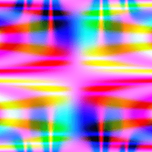
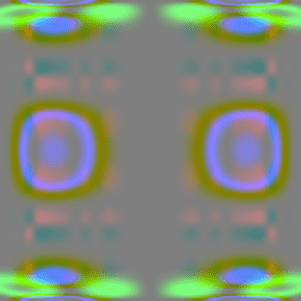
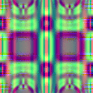
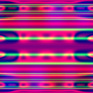
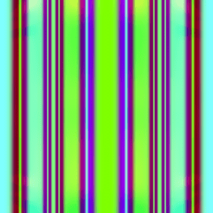
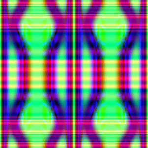
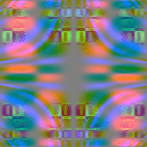
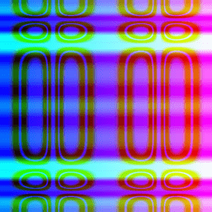
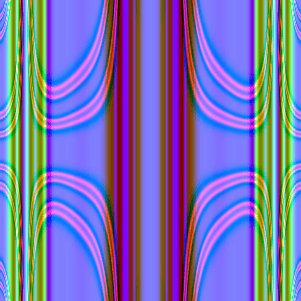
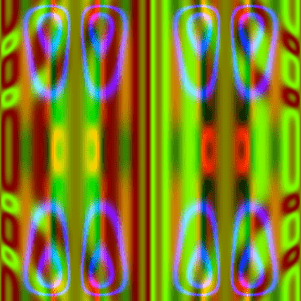
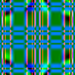
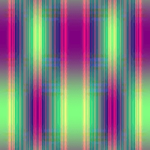
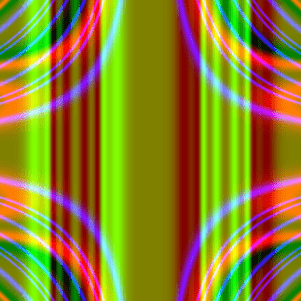
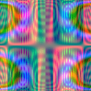
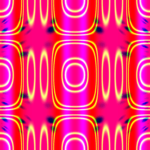
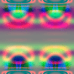
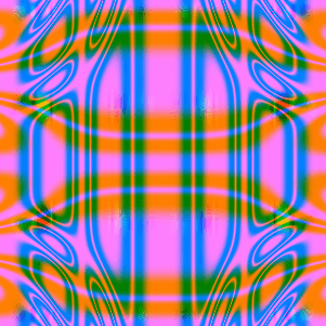
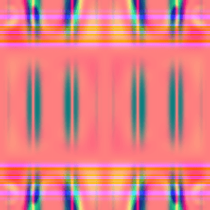
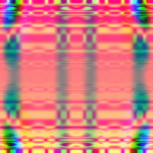
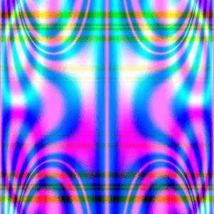
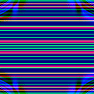
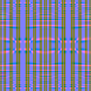
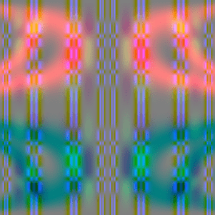
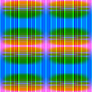
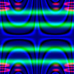
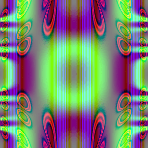
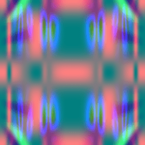
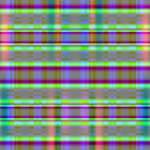
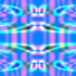
Indeed, the designs are all rather psychedelic, and the layers of color are completely unrelated. It would be an interesting venture to write a program which, given an image of something (pretend it’s a simple image containing some shapes), constructs expression trees that are consistent with the curves and lines in the image. Until next time, enjoy these pictures!
Gallery


Want to respond? Send me an email, post a webmention, or find me elsewhere on the internet.