Numerical Integration

Rectangles, Trapezoids, and Simpson’s

I just wrapped up a semester of calculus TA duties, and I thought it would be fun to revisit the problem of integration from a numerical standpoint. In other words, the goal of this article is to figure out how fast we can approximate the definite integral of a function $ f:\mathbb{R} \to \mathbb{R}$. Intuitively, a definite integral is a segment of the area between a curve $ f$ and the $ x$-axis, where we allow area to be negative when $ f(x) < 0$.

If any of my former students are reading this, you should note that we will touch on quite a number of important ideas from future calculus courses, but until you see them in class, the proofs may seem quite mystical.

As usual, the source code for this post is available on this blog’s Github page.

The Baby Integral

Let’s quickly recall the definition of an integral $ \int_a^b f(x) dx$:

Definition: Let $ P = \left \{ [a_i, b_i] \right \}_{i = 1}^n$ be a partition of an interval $ [a,b]$ into $ n$ sub-intervals, let $ \Delta x_i = b_i – a_i$ be the length of each interval, and let $ \widehat{x_i}$ be a chosen point inside $ [a_i,b_i]$ (which we call a tag). Then a Riemann sum of $ f$ from $ a$ to $ b$ is a sum

$ \displaystyle R(f, P) = \sum_{i = 1}^n f(\widehat{x_i}) \Delta x_i$.

Geometrically, a Riemann sum approximates the area under the curve $ f$ by using sufficiently small rectangles whose heights are determined by the tagged points. The terms in the sum above correspond to the areas of the approximating rectangles.

We note that the intervals in question need not have the same lengths, and the points $ \widehat{x_i}$ may be chosen in any haphazard way one wishes. Of course, as we come up with approximations, we will pick the partition and tags very deliberately.

Definition: The integral $ \displaystyle \int_a^b f(x) dx$ is the limit of Riemann sums as the maximum length of any sub-interval in the partition goes to zero. In other words, for a fixed partition $ P$ let $ \delta_P = \max_i(\Delta x_i)$. Then

Another way to put this definition is that if you have any sequence of partitions $ P_k$ so that $ \delta_{P_k} \to 0$ as $ k \to \infty$, then the integral is just the limit of Riemann sums for this particular sequence of partitions.

Our first and most naive attempt at computing a definite integral is to interpret the definition quite literally. The official name for it is a left Riemann sum. We constrain our partitions $ P$ so that each sub-interval has the same length, namely $ \Delta x = (b-a)/n$. We choose our tags to be the leftmost points in each interval, so that if we name each interval $ [a_i, b_i]$, we have $ \widehat{x_i} = a_i$. Then we simply use a large enough value of $ n$, and we have a good approximation of the integral.

For this post we used Mathematica (gotta love those animations!), but the code to implement this is quite short in any language:

LeftRiemannSum[f_, n_, a_, b_] :=
 Module[{width = (b-a)/n},
  N[width * Sum[f[a + i*width], {i, 0, n-1}]]
 ];

Note that we may factor the constant “width” out of the sum, since here it does not depend on the interval. The only other detail is that Mathematica leaves all expressions as exact numbers, unless they are wrapped within a call to N[ ], which stands for “numerical” output. In most general languages numerical approximations are the default.

The computational complexity should be relatively obvious, as we require “one” computation per interval, and hence $ n$ computations for $ n$ intervals. (Really, it depends on the cost of evaluating $ f(x)$, but for the sake of complexity we can assume computing each term is constant.) And so this algorithm is $ O(n)$.

However, we should note that our concern is not necessarily computational complexity, but how fast the sum converges. In other words, we want to know how large $ n$ needs to be before we get a certain number of decimal places of accuracy.

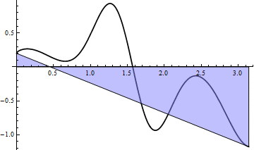
For all of our tests and visualizations, we will use the following arbitrarily chosen, but sufficiently complicated function on $ [0, \pi]$:

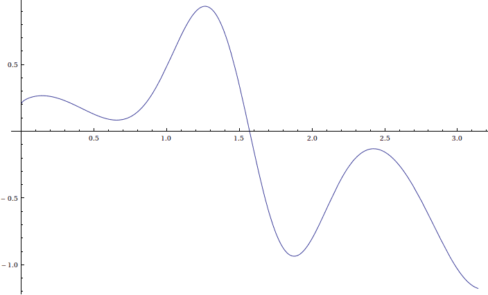
For n = 15, we have the following left Riemann sum:

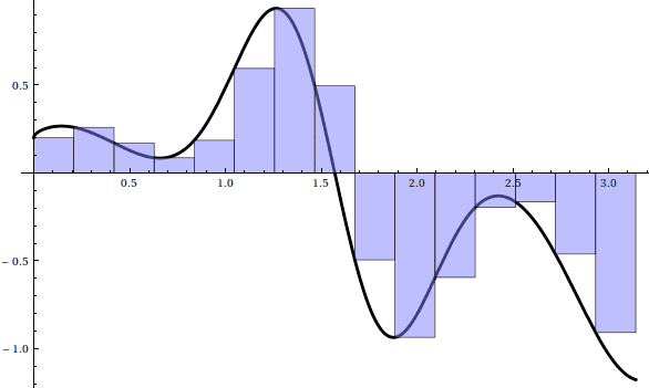
Here’s an animation of the sum as $ n \to 100$:

Unfortunately, it seems that on the regions where $ f$ is increasing, that portion of the Riemann sum is an underestimate, and where $ f$ is decreasing, the Riemann sum is an overestimate. Eventually this error will get small enough, but we note that even for $ n = 10,000$, the sum requires almost 7 seconds to compute, and only achieves 3 decimal places of accuracy! From a numerical standpoint, left Riemann sums converge slower than paint dries and are effectively useless. We can certainly do better.

More Geometric Intuition

Continuing with the geometric ideas, we could conceivably pick a better tag in each sub-interval. Instead of picking the left (or right) endpoint, why not pick the midpoint of each sub-interval? Then the rectangles will be neither overestimates nor underestimates, and hence the sums will be inherently more accurate. The change from a left Riemann sum to a midpoint Riemann sum is trivial enough to be an exercise for the reader (remember, the source code for this post is available on this blog’s Github page). We leave it as such, and turn to more interesting methods.

Instead of finding the area of a rectangle under the curve, let’s use a trapezoid whose endpoints are both on the curve. (Recall the area of a trapezoid, if necessary) We call this a trapezoid sum, and a first attempt at the code is not much different from the left Riemann sum:

TrapezoidSum[f_, n_, a_, b_] :=
 Module[{width = (b-a)/n},
  N[width * Sum[1/2 (f[a + i*width] + f[a + (i+1)*width]),
     {i, 0, n-1}]]
 ];

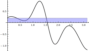
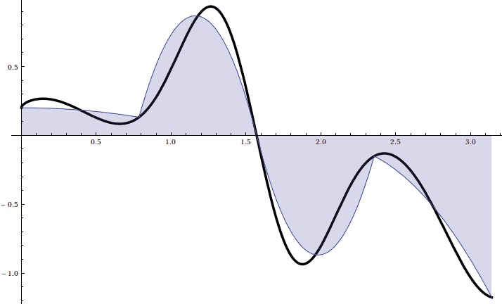
Here is a picture for $ n = 15$:

And an animation as $ n \to 100$:

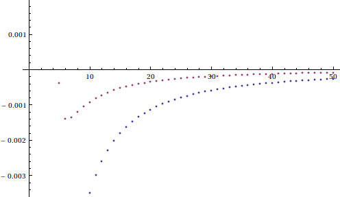
The animation hints that this method converges much faster than left Riemann sums, and indeed we note that for $ n = 100$, the sum requires a mere .16 seconds, yet achieves the three decimal places of accuracy for which the left Riemann sum required $ n = 10,000$. This method appears to be a drastic improvement, and indeed plotting the accuracy of left Riemann sums against trapezoid sums gives a nice indication:

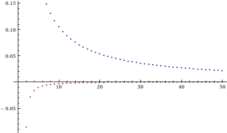
Now that is quite an improvement!

Going back to the code, the computational complexity is again $ O(n)$, but we note that at a micro-efficiency level, we are being a bit wasteful. We call the function $ f$ twice for each trapezoid, even when adjacent trapezoids share edges and hence base heights. If a call to $ f$ is relatively expensive (and it just so happens that calls to Sin, Cos, Exp are somewhat expensive), then this becomes a significant issue. We leave it as an exercise to the adventurous reader to optimize the above code, so that no superfluous calls to $ f$ are made (hint: surround the function $ f$ with a cache, so that you can reuse old computations).

Before we move on to our final method for this post, we will take a no-so-short aside to give a proof of how accurate the trapezoid rule is. In fact, we will give an upper bound on the error of trapezoid sums based solely on $ n$ and easy properties of $ f$ to compute. In it’s raw form, we have the following theorem:

Theorem: Supposing $ f: [a,b] \to \mathbb{R}$ is thrice differentiable, let $ h = (b-a)/n$, let $ a_i$ be $ a + (i-1)h$, and let $ T_n(f)$ be a trapezoidal approximation of $ f$ with $ n$ trapezoids, as above. Then

Proof. Let $ \varphi_i : [0,h] \to \mathbb{R}$ be defined by

We claim that $ \sum \limits_{i=1}^n \varphi_i(h) = T_n(f) – \int_a^b f(x) dx$, and one can see this by simply expanding the sum according to the definition of $ \varphi_i$. Now we turn to the question of bounding $ \varphi_i$ on $ [0,h]$.

We note $ \varphi_i(0) = 0$, and by the fundamental theorem of calculus:

Furthermore, $ \varphi_i'(0) = 0$ as is evident by the above equation, and differentiating again gives us

With again $ \varphi_i”(0) = 0$.

As $ f”$ is continuous, the extreme-value theorem says there exist bounds for $ f$ on $ [a,b]$. We call the lower one $ m$ and the upper $ M$, so that

Taking definite integrals twice on $ [0,t]$, we get

Then the sum of all the $ \varphi_i(h)$ may be bounded by

The definition of $ h$ and some simplification gives

And from here we note that by continuity, $ f”(x)$ obtains every value between its bounds $ m, M$, so that for some $ c \in [a,b], f”(c)$ obtains the value needed to make the middle term equal to $ \frac{b-a}{12}h^2 f”(c)$, as desired.

As a corollary, we can bound the magnitude of the error by using the larger of $ |m|, |M|$, to obtain a fixed value $ B$ such that

So what we’ve found is that the error of our trapezoidal approximation (in absolute value) is proportional to the function $ 1/n^2$. There is a similar theorem about the bounds of a left Riemann sum, and we leave it as an exercise to the reader to find and prove it (hint: use a similar argument, or look at the Taylor expansion of $ f$ at the left endpoint).

Interpolating Polynomials and Simpson’s Rule

One way to interpret the left Riemann sum is that we estimate the integral by integrating a step function which is close to the actual function. For the trapezoidal rule we estimate the function by piecewise lines, and integrate that. Naturally, our next best approximation would be estimating the function by piecewise quadratic polynomials. To pick the right ones, we should investigate the idea of an interpolating polynomial.

Following the same pattern, given one point there is a unique constant function (degree zero polynomial) passing through that point. Given two points there is a unique line (degree one) which contains both. We might expect that given $ n+1$ points in the plane (in general position), there is a unique degree $ n$ polynomial passing through them.

For three points, $ (x_1, y_1), (x_2, y_2), (x_3, y_3)$ we may concoct a working curve as follows (remember $ x$ is the variable here)

Notice that each of the terms are 2nd degree, and plugging in any one of the three given $ x$ values annihilates two of the terms, and gives us precisely the right $ y$ value in the remaining term. We may extend this in the obvious way to establish the interpolating polynomial for a given set of points. A proof of uniqueness is quite short, as if $ p, q$ are two such interpolating polynomials, then $ p-q$ has $ n+1$ roots, but is at most degree $ n$. It follows from the fundamental theorem of algebra that $ p-q$ must be the zero polynomial.

If we wish to approximate $ f$ with a number of these quadratics, we can simply integrate the polynomials which interpolate $ (a_i, f(a_i)), (a_{i+1}, f(a_{i+1})), (a_{i+2}, f(a_{i+2}))$, and do this for $ i = 1, 3, \dots, n-2$. This is called Simpson’s Rule, and it gives the next level of accuracy for numerical integration.

With a bit of algebra, we may write the integrals of the interpolating polynomials in terms of the points themselves. Without loss of generality, assume the three points are centered at 0, i.e. the points are $ (- \delta, y_1), (0, y_2), (\delta, y_3)$. This is fine because shifting the function left or right does not change the integral. Then the interpolating polynomial is (as above),

$ \displaystyle p(x) = \frac{(x+\delta)(x)}{2 \delta^2}y_3 + \frac{(x+\delta)(x-\delta)}{-\delta^2}y_2 + \frac{(x)(x-\delta)}{2 \delta^2}y_1$.

Integrating this over $ [-\delta, \delta]$ and simplifying gives the quantity

$ \displaystyle \int_{-\delta}^{\delta} p(x) dx = \frac{\delta}{3}(y_1 + 4y_2 + y_3)$.

And so we may apply this to each pair of sub-intervals (or work with the midpoints of our $ n$ sub-intervals), to get our quadratic approximation of the entire interval. Note, though that as we range over all sub-intervals, the two endpoints will be counted twice, so our entire approximation is

Translating this into code is as straightforward as one could hope:

SimpsonsSum[f_, n_, a_, b_] :=
 Module[{width = (b-a)/n, coefficient},
  coefficient[i_?EvenQ] = 2;
  coefficient[i_?OddQ] = 4;
  N[width/3 * (f[a] + f[b] +
     Sum[coefficient[i] * f[a + i*width], {i, 1, n-1}])]
 ];

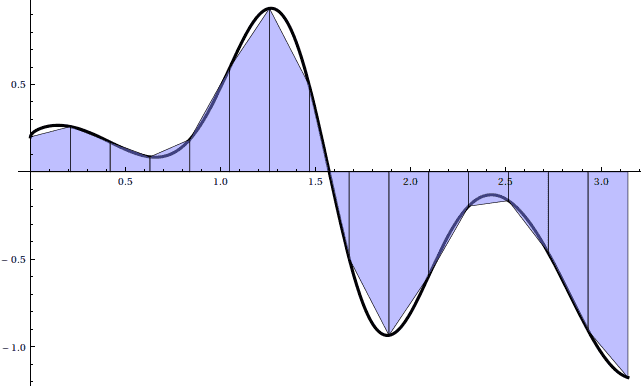
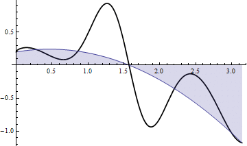
As usual, here is a picture for $ n = 8$:

And an animation showing the convergence:

There is a similar bound for Simpson’s Rule as there was for the trapezoid sums. Here it is:

Theorem: Supposing $ f$ is five times differentiable, and let $ B$ be the maximum of the values $ |f^{(4)}(c)|$ for $ c$ in $ [a,b]$. Then the magnitude of the difference between the true integral $ \int_a^b f(x) dx$ and the Simpson’s Rule approximation with $ n$ interpolated polynomials is at most

The proof is similar in nature to the proof for trapezoid sums, but requires an annoying amount of detail. It’s quite difficult to find a complete proof of the error estimate for reference. This is probably because it is a special case of a family of Newton-Cotes formulas. We leave the proof as a test of gumption, and provide a reference to a slightly more advanced treatment by Louis A. Talman.

As an easier cop-out, we show a plot of the convergence of Simpson’s Rule versus the trapezoid sums:

Judging by the graph, the improvement from trapezoid sums to Simpson’s rule is about as drastic as the improvement from Riemann sums to trapezoid sums.

Final Thoughts, and Future Plans

There are a host of other integral approximations which fall in the same category as what we’ve done here. Each is increasingly accurate, but requires a bit more computation in each step, and the constants involved in the error bound are based on larger and larger derivatives. Unfortunately, in practice it may hard to bound large derivatives of an arbitrary function, so confidence in the error bounds for simpler methods might be worth the loss of efficiency for some cases.

Furthermore, we always assumed that the length of each sub-interval was uniform across the entire partition. It stands to reason that some functions are wildly misbehaved in small intervals, but well-behaved elsewhere. Consider, for example, $ \sin(1/x)$ on $ (0, \pi)$. It logically follows that we would not need small intervals for the sub-intervals close to $ \pi$, but we would need increasingly small intervals close to 0. We will investigate such methods next time.

We will also investigate the trials and tribulations of multidimensional integrals. If we require 100 evenly spaced points to get a good approximation of a one-dimensional integral, then we would require $ 100^2$ evenly spaced points for a two-dimensional integral, and once we start working on interesting problems in 36,000-dimensional space, integrals will require $ 100^{36,000}$ evenly spaced points, which is far greater than the number of atoms in the universe (i.e., far exceeds the number of bits available in all computers, and hence cannot be computed). We will investigate alternative methods for evaluating higher-dimensional integrals, at least one of which will be based on random sampling.

Before we close, we note that even today the question of how to approximate integrals is considered important research. Within the last twenty years there have been papers generalizing these rules to arbitrary spaces, and significant (“clever”) applications to the biological sciences. Here are two examples: Trapezoidal rules in Sobolev spaces, and Trapezoidal rule and Simpson’s rule for “rough” continuous functions. Of course, as we alluded to, when dimension goes up integrals become exponentially harder to compute. As our world is increasingly filled with high-dimensional data, rapid methods for approximating integrals in arbitrary dimension is worth quite a bit of money and fame.

Until next time!