Kolmogorov Complexity – A Primer

The Complexity of Things

Previously on this blog (quite a while ago), we’ve investigated some simple ideas of using randomness in artistic design (psychedelic art, and earlier randomized css designs), and measuring the complexity of such constructions. Here we intend to give a more thorough and rigorous introduction to the study of the complexity of strings. This naturally falls into the realm of computability theory and complexity theory, and so we refer the novice reader to our other primers on the subject (Determinism and Finite Automata, Turing Machines, and Complexity Classes; but Turing machines will be the most critical to this discussion).

The Problem with Randomness

What we would really love to do is be able to look at a string of binary digits and decide how “random” it is. On one hand, this is easy to do at a high level. A child would have no difficulty deciding which of the following two strings is more random:

10101010101010101010101010101010101010101010101010
00011101001000101101001000101111010100000100111101

And yet, by the immutable laws of probability, each string has an equal chance ($ 2^{-50}$) in being chosen at random from all sequences of 50 binary digits. So in a sense, the huge body of mathematics underlying probability has already failed us at this basic juncture because we cannot speak of how random one particular outcome of an experiment is. We need a new notion that overcomes this difficulty.

Definition: The Kolmogorov complexity of a string $ w$, denoted $ K(w)$ is the length of the shortest program which outputs $ w$ given no input.

While this definition is not rigorous enough to be of any use (we will reformulate it later), we can easily see why the first of the two strings above is less random. We can write a very short Python program that outputs it:

print "01" * 25

On the other hand, it is not hard to see that the shortest program that produces the second string is

print "00011101001000101101001000101111010100000100111101"

The dutiful reader will cry out in protest. How do you know that’s the shortest program? Why restrict to Python? This whole discussion is so arbitrary!

Indeed, this is probably not the strictly shortest Python program that prints out the string. In the following we’ll work entirely in binary, so the picky reader should interpret this as a print command referring to a block of binary memory. We will reify these ideas in full rigor shortly, but first let us continue with this naivete to make the coming definitions a bit easier to parse.

If we abstract away the lengths of these strings, we see that the length of the first program is $ O(1) + \log(n)$, since we need $ \log(n)$ bits to represent the number $ n/2$ in the string product. On the other hand, the second string has a program length of $ O(1) + n$, as we require the entire output string as program text.

This intuition would lead us to define a sequence of length $ n$ to be random if it has Kolmogorov complexity at least $ n$. One way to interpret this is: a string is “random” if the shortest program that outputs the string basically encodes the entire string in its source code.

We can extend this idea to talk about relative complexity. Specifically, we can speak of Python programs which accept input, and compute their output based on that input. For instance, the first of the two strings above has the program:

n = input()
print "01" * n/2

With respect to the input “50”, we see that the first string has constant complexity (indeed, this is also true of many numbers, such as 25). In other words, the string “50” contains a lot of information about the string we wish to generate (it’s length).

On the other hand, the same technique still won’t work for the second string. Even though it has length 50, that is not enough information to determine the contents of the string, which vary wildly. So the shortest program is still (probably) the one which prints out the string verbatim.

In the future, we plan to revisit the idea of relative complexity in the context of machine learning and classification; briefly, two items are similar if one has low complexity relative to the other. But for now, let us turn to the more precise definitions.

Actual Kolmogorov Complexity

We keep saying of the second string above that the shortest program is probably the one which prints the string verbatim. In fact, short of testing every single python program of shorter length, we will never know if this is true! Even if we did, our following definitions will make that discovery irrelevant. More generally, it’s an important fact that Kolmogorov complexity is an uncomputable function. That is, there is no Turing machine $ M$ which accepts as input a word $ w$ and produces its Kolmogorov complexity as output. In order to prove such miraculous things, we need to formalize the discussion in the context of Turing machines.

Let us fix a universal programming language $ L$ and speak of the Kolmogorov complexity with respect to $ L$:

Definition: The Kolmogorov complexity of a string $ w$ with respect to $ L$, denoted $ K_L(w)$ is the shortest program written in the language $ L$ which produces $ w$ as output. The conditional Kolmogorov complexity with respect to a string $ x$, denoted $ K_L(w | x)$ (spoken $ w$ given $ x$, as in probability theory), is the length of the shortest program which, when given $ x$ as input, outputs $ w$.

Before we can prove that this definition is independent of $ L$ (for all intents and purposes), we need a small lemma, which we have essentially proved already:

Lemma: For any strings $ w,x$ and any language $ L$, we have $ K_L(w | x) \leq |w| + c$ for some constant $ c$ independent of $ w, x$, and $ K_L(w) \leq |w| + c’$ for some constant $ c’$ independent of $ w$.

Proof. The program which trivially outputs the desired string has length $ |w| + c$, for whatever constant number of letters $ c$ is required to dictate that a string be given as output. This is clearly independent of the string and any input. $ \square$

It is not hard to see that this definition is invariant under a choice of language $ L$ up to a constant factor. In particular, let $ w$ be a string and fix two languages $ L, L’$. As long as both languages are universal, in the sense that they can simulate a universal Turing machine, we can relate the Kolmogorov complexity of $ w$ with respect to both languages. Specifically, one can write an interpreter for $ L$ in the language of $ L’$ and vice versa. Readers should convince themselves that for any two reasonable programming languages, you can write a finite-length program in one language that interprets and executes programs written in the other language.

If we let $ p$ be the shortest program written in $ L$ that outputs $ w$ given $ x$, and $ i$ be the interpreter for $ L$ written in $ L’$, then we can compute $ w$ given the input $ \left \langle p, x \right \rangle$ by way of the interpreter $ i$. In other words, $ K_L(w | px) \leq |i|$.

$ K_{L’}(w | x) \leq |p| + c + |i| = K_L(w | x) + c + |i| = K_L(w | x) + O(1)$

Another easy way to convince oneself of this is to imagine one knows the language $ L’$. Then the program would be something akin to:

input x
run the interpreter i on the program p with input x

Our inequalities above just describe the length of this program: we require the entire interpreter $ i$, and the entire program $ p$, to be part of the program text. After that, it’s just whatever fixed constant amount of code is required to initialize the interpreter on that input.

We call this result the invariance property of Kolmogorov complexity. And with this under our belt, we may speak of the Kolmogorov complexity of a string. We willingly ignore the additive constant difference which depends on the language chosen, and we may safely work exclusively in the context of some fixed universal Turing machine (or, say, Python, C, Racket, or Whitespace; pick your favorite). We will do this henceforth, denoting the Kolmogorov complexity of a string $ K(w)$.

Some Basic Facts

The two basic facts we will work with are the following:

  • There are strings of arbitrarily large Kolmogorov complexity.
  • Most strings have high complexity.

And we will use these facts to prove that $ K$ is uncomputable.

The first point is that for any $ n$, there is a string $ w$ such that $ K(w) \geq n$. To see this, we need only count the number of strings of smaller length. For those of us familiar with typical combinatorics, it’s just the Pigeonhole Principle applied to all strings of smaller length.

Specifically, there is at most one string of length zero, so there can only be one string with Kolmogorov complexity zero; i.e., there is only one program of length zero, and it can only have one output. Similarly, there are two strings of length one, so there are only two strings with Kolmogorov complexity equal to one. More generally, there are $ 2^i$ strings of length $ i$, so there are at most $ \sum_{i = 0}^{n-1} 2^i$ strings of Kolmogorov complexity less than $ n$. However, as we have seen before, this sum is $ 2^n – 1$. So there are too many strings of length $ n$ and not enough of smaller length, implying that at least one string of length $ n$ has Kolmogorov complexity at least $ n$.

The second point is simply viewing the above proof from a different angle: at least 1 string has complexity greater than $ n$, more than half of the $ 2^n$ strings have complexity greater than $ n-1$, more than three quarters of the strings have complexity greater than $ n-2$, etc.

Rigorously, we will prove that the probability of picking a string with $ K(x) \leq n – c – 1$ is smaller than $ 1/2^c$. Letting $ S$ be the set of all such strings, we have an injection $ S \hookrightarrow $ the set of all strings of length less than $ n – c- 1$, and there are $ 2^{n-c} – 1$ such strings, so $ |S| \leq 2^{n-c} – 1$, giving the inequality:

$ \displaystyle \frac{|S|}{2^n} \leq \frac{2^{n-c} – 1}{2^n} = \frac{1}{2^c} – \frac{1}{2^n} < \frac{1}{2^c}$

In other words, the probability that a randomly chosen string $ w$ of length $ n$ has $ K(w) \geq n-c$ is at least $ 1 – 1/2^c$.

The strings of high Kolmogorov complexity have special names.

Definition: We call a string $ w$ such that $ K(w) \geq |w|$ a Kolmogorov random string, or an incompressible string.

This name makes sense for two reasons. First, as we’ve already mentioned, randomly chosen strings are almost always Kolmogorov random strings, so the name “random” is appropriate. Second, Kolmogorov complexity is essentially the ideal compression technique. In a sense, strings with high Kolmogorov complexity can’t be described in any shorter language; such a language would necessarily correspond to a program that decodes the language, and if the compression is small, so is the program that decompresses it (these claims are informal, and asymptotic).

Uncomputability

We will now prove the main theorem of this primer, that Kolmogorov complexity is uncomputable.

Theorem: The Kolmogorov complexity function $ w \mapsto K(w)$ is uncomputable.

Proof. Suppose to the contrary that $ K$ is computable, and that $ M$ is a Turing machine which computes it. We will construct a new Turing machine $ M’$ which computes strings of high complexity, but $ M’$ will have a short description, giving a contradiction.

Specifically, $ M’$ iterates over the set of all binary strings in lexicographic order. For each such string $ w$, it computes $ K(w)$, halting once it finds a $ w$ such that $ K(w) \geq |w| = n$. Then we have the following inequality:

$ n \leq K(w) \leq \left | \left \langle M’, n \right \rangle \right | + c$

Here, the angle bracket notation represents a description of the tuple $ (M’, n)$, and $ c$ is a constant depending only on $ M’$, which is fixed. The reason the inequality holds is just the invariance theorem: $ \left \langle M’, n \right \rangle$ is a description of $ w$ in the language of Turing machines. In other words, the universal Turing machine which simulates $ M’$ on $ n$ will output $ w$, so the Kolmogorov complexity of $ w$ is bounded by the length of this description (plus a constant).

Then the length of $ \left \langle M’, n \right \rangle$ is at most $ \log(n) + \left | \left \langle M’ \right \rangle \right | + c’$ for some constant $ c’$, and this is in turn $ \log(n) + c”$ for some constant $ c”$ (as the description of $ M’$ is constant). This gives the inequality

$ n \leq \log(n) + c”$

But since $ \log(n) = o(n)$, we may pick sufficiently large $ n$ to achieve a contradiction. $ \square$

We can interpret this philosophically: it is impossible to tell exactly how random something is. But perhaps more importantly, this is a genuinely different proof of uncomputability from our proof of the undecidability of the Halting problem. Up until now, the only way we could prove something is uncomputable is to reduce it to the Halting problem. Indeed, this lends itself nicely to many new kinds of undecidability-type theorems, as we will see below.

The reader may ask at this point, “Why bother talking about something we can’t even compute!?” Indeed, one might think that due to its uncomputability, Kolmogorov complexity can only provide insight into theoretical matters of no practical concern. In fact, there are many practical applications of Kolmogorov complexity, but in practice one usually gives a gross upper bound by use of the many industry-strength compression algorithms out there, such as Huffman codes. Our goal after this primer will be to convince you of its remarkable applicability, despite its uncomputability.

Consequences of Uncomputability and Incompressibility

One immediate consequence of the existence of incompressible strings is the following: it is impossible to write a perfect lossless compression algorithm. No matter how crafty one might be, there will always be strings that cannot be compressed.

But there are a number of other, more unexpected places that Kolmogorov complexity fills a niche. In computational complexity, for instance, one can give a lower bound on the amount of time it takes a single-tape Turing machine to simulate a two-tape Turing machine. Also in the realm of lower bounds, one can prove that an incompressible string $ w$ of length $ 2^n$, which can be interpreted as a boolean function on $ n$ variables, requires $ \Omega(2^n/n)$ gates to express as a circuit.

It also appears outside of theoretical computer science. In, for instance, the study of entropy in dynamical systems (specifically, thermodynamics), one can make the following pictorial remark:

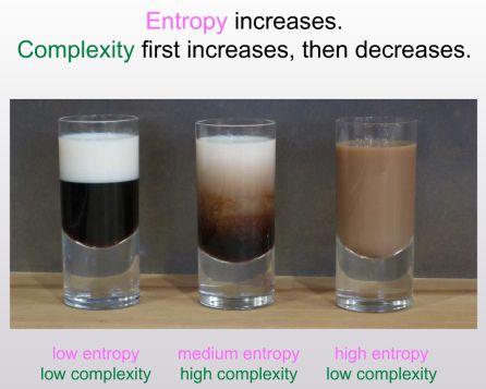
In fact, the author of this image, Scott Aaronson (whom we’ve seen before in our exploration of the Complexity Zoo) even proposes an empirical test of this fact: simulate a discretized coffee cup and try to compress the data at each step, graphing the resulting lengths to see the trends. This even sounds like a good project for this blog!

The applications don’t end there, though. Researchers have used the theory of Kolmogorov complexity to tackle problems in machine learning, clustering, and classification. Potentially, any subject which is concerned with relating pieces of information could benefit from a Kolmogorov-theoretic analysis.

Finally, we give a proof that the existence of Kolmogorov complexity provides an infinite number of mathematical statements which are unprovable.

Theorem: Fix a formalization of mathematics in which the following three conditions hold:

  • If a statement is provable then it is true.
  • Given a proof and a statement, it is decidable whether the proof proves the statement.
  • For every binary string $ x$ and integer $ k$, we can construct a statement $ S(x,k)$ which is logically equivalent to “the Kolmogorov complexity of $ x$ is at least $ k$”.

Then there is some constant $ t$ for which all statements $ S(x,k)$ with $ k > t$ are unprovable.

Proof. We construct an algorithm to find such proofs as follows:

On an input k,
Set m equal to 1.
Loop:
   for all strings x of length at most m:
      for all strings P of length at most m:
         if P is a proof of S(x,k), output x and halt
   m = m+1

Suppose to the contrary that for all $ k$ there is an $ x$ for which the statement $ S(x,k)$ is provable. It is easy to see that the algorithm above will find such an $ x$. On the other hand, for all such proofs $ P$, we have the following inequality:

$ k \leq K(x) \leq \left | \left \langle M, k \right \rangle \right | + c = \log(k) + c’$

Indeed, this algorithm is a description of $ x$, so its length gives a bound on the complexity of $ x$. Just as in the proof of the uncomputability of $ K$, this inequality can only hold for finitely many $ k$, a contradiction. $ \square$

Note that this is a very different unprovability-type proof from Gödel’s Incompleteness Theorem. We can now construct with arbitrarily high probability arbitrarily many unprovable statements.

Look forward to our future posts on the applications of Kolmogorov complexity! We intend to explore some compression algorithms, and to use such algorithms to explore clustering problems, specifically for music recommendations.

Until then!

45 thoughts on “Kolmogorov Complexity – A Primer

  1. I stopped reading at your “Definition” paragraph as it occurred to me a trivial program like this invalidates your “n bits to store the second string” argument. You may have had a valid point to make later on, but I was sufficiently distracted by your poor example not to read any further:

    “000”+bin(128141569638717)[2:].rjust(8,’0′)

    • You’ve just said that a string of n zeros and ones can be represented with \log(n) digits. So the Kolmogorov complexity of a binary string is bounded by \log(n) + c for some constant c independent of n. Fine. That’s an elementary exercise, and only tangentially related to my point. What if instead of Python you had to write this program in some restricted assembly language, and the output was just a binary stream? Then would you agree that the shortest program is just to output the string itself? In reality we do this mathematics on a Turing machine, which doesn’t have “bin()” or “rjust()”. And in that context, your program would require the entire Python interpreter (and string formatting library) to evaluate this program. That would certainly push the Kolmogorov complexity far above 50 characters.

      The point is that it’s not obvious how to compress that string more than you just did, and you actually didn’t compress it at all if we work entirely in binary. So please, read on! The enlightening parts are toward the end, not in the pedantic overview.

    • “”””I stopped reading at your “Definition” paragraph as it occurred to me a trivial program like this invalidates your “n bits to store the second string” argument. You may have had a valid point to make later on, but I was sufficiently distracted by your poor example not to read any further””””

      Or maybe it was just your ADD. Or it could be the need to make a cocky statement about a introductory (“a primer”) text. I guess the main reason is you weren’t loved enough as a child and/or bullied at school.

      You don’t like those answers? Fine. I don’t like the arrogant “I’ve stopped reading after…” pissing on another guy’s post either.

    • “””You may have had a valid point to make later on, but I was sufficiently distracted by your poor example not to read any further:”””

      LOL… your example is even poorer:

      a) misses the point
      b) fixates on a triviality of the implementation
      c) provides no value

      Basically, you’re just a “well actually” guy:

      http://tirania.org/blog/archive/2011/Feb-17.html

      • I’d prefer to keep the comments somewhat flame-free, so I’m only allowing this comment because I like the linked article on Well Actually Guys 🙂

    • So you proved that you are an idiot that is unable to see the big picture and is distracted by every little thing he notices.

      Rarely was any insight gained by someone saying “I stopped reading at …”. Except for the insight that the guy wants to play it oh-so-clever, that is.

  2. I don’t suppose that latex code after “we see that the length of the first program is” was supposed to show up the published article…

  3. This comment is incorrect:

    “And yet, by the immutable laws of probability, each string has an equal chance (2^{-50}) in being chosen at random from all sequences of 50 binary digits. So in a sense, the huge body of mathematics underlying probability has already failed us …”

    You can easily construct the distribution for the number of instances of “01” that a fifty bit substring will have if each bit is generated bernoulli (iid) with p=0.5. And if you do you will find that your “non-random” string will be far less likely under this distribution than your apparently random string

    • I’m really really sad that I don’t know more about statistical theory to agree or disagree with you, so I’ll assume you’re right. Should I have said, “chosen at random from a uniform distribution”? That is what I meant.

      I think the point I was trying to make is still valid: we can’t talk about the randomness of an outcome (or it’s particularly difficult to do so) with the language of probability theory.

    • There’s nothing incorrect about j2kun’s statement. Generating each bit independently with P(bit_i = 1) = .5 will result in a uniform distribution over all strings. Each string will have probability mass 2^-50.

      You can calculate a statistic of a string T(X) if you want, like your example: T(X) = count(“10”, X).
      But when you look at P(T(X) = k) for some k, you’re grouping together multiple strings (the equivalence class {X | T(X) = k}) under the same probability mass.
      You will come up with a non-uniform distribution *for that statistic*, under which P(T(X) = 13) > P(T(X) = 25).
      But when T(a)=13 and T(b)=25 like it does for the “random” and “non-random” strings respectively, that doesn’t mean that P(a) > P(b).
      It means P(strings “like” a) > P(strings “like” b), with the meaning of “like” depending on T.
      You’ll find that once you multiply in the conditional probability P(X) = P(X | T(X)=k) * P(T(X)=k) you’ll get back to uniform.
      And there’s no reason to prefer your statistic T over some other statistic.
      E.g. T_2(X) = count(“1”, X) or T_3(X) = count(“0”, X) both assign higher probability to b’s class.

      Nice article, btw 🙂

  4. Interesting post. Was a bit unclear on how you went from || to log(n) + c though. After looking it up, it seems to me to follow from some result inside your probability discussion, but it wasn’t clear to me on first glance.

  5. Nice article ! If I may, there seems to be a glitch near “we see that the length of the first program is”.

  6. print “01” * 25

    n = input()
    print “01” * n/2

    For the first one above, you say that log(n) bits are needed to represent n/2 (25 here), but the first line of the second one is of constant complexity. When you take into account that integers in computers are generally of bounded range. A correct matching implementation would also use log(n) memory and time for the integer processing.

    • I think you’re misunderstanding. On one hand, we don’t care about the space or time requirements of the machine when analyzing Kolmogorov complexity. All we care about is the length of a description of the program (here, the number of bits in the binary representation of the program text). The program could (and in many cases of extreme compression, it does) require exponential time to compute. If we let n get significantly larger than 50, then storing the number n verbatim in the program text requires log(n) bits.

      Moreover, we are not concerned with the realities of integer representations in computers. This discussion is in the context of a Turing machine, in which integers are unbounded (binary) quantities.

      There is another more recent (and apparently very applicable) variant of Kolmogorov complexity called time-bounded Kolmogorov complexity, for which we require the computation happens in polynomial time. This has strong connections to things like circuit complexity (roughly, the two are equivalent).

  7. I’m no expert, but information theory answers the question of “randomness” more simply, intuitively and rigorously.

    This notion of Kolmogorov Complexity doesn’t seem to add any additional value.

    • I think you’re being a bit naive… This is established mathematics for a good reason, and you’re saying that having a different perspective on a topic adds no value. You’re right that the two theories are related, but from my basic reading on information theory, it’s concerned with the entropy of information transmitted in the presence of noise. Indeed, Kolmogorov complexity is sometimes considered a sub-field of information theory, but it can certainly be developed independently.

      And Kolmogorov complexity does more than just add perspective. Like I wrote, you can generate results on incompleteness of logical systems, talk about universal distributions, give important theoretical lower bounds on circuit complexity and the running time of Turing machines. And there are many practical applications as well to fields like machine learning, compression algorithms, and a variety of other topics. But you don’t have to take my word for it; my goal with this blog is to show you such applications and convince you of its usefulness. So look forward to that.

  8. There is a touch of circularity in the coffee cup experiment. The tacit assumption that our compression algorithms are *any good* is not necessarily true. Therefore a chart of compressing the state of the simulation could be taken as a measure of our algorithms, rather than some proof of irreducible complexity.

    One trivial way to ‘compress’ the state of the coffee cup simulation at any time is for me to represent any intermediate state as an ordered pair consisting of the program itself (a string), and the point in time you want to represent (a number). These two pieces of information are certainly sufficient to indicate the state of the simulation, and the length of this representation is constant for all time. This might seem like a pedantic trick, and not at all what we typically mean by ‘compression’, but I think it has profound implications.

    For example, there seems to be an assumption that programs are like machines that operate on some mutable data structure, leaving a ‘residue’ (state) of their operation up to that point. In the coffee cup simulation, this residue is, say, a graphic image of what the coffee looks like at any time. The program may have a lower entropy representation of this image, but I think we can assume without loss of generality that the low entropy representation of the image is isomorphic to it.

    Another implication is that it is exceedingly hard to infer a program from it’s output. That is, in some sense, the critical distinction between a program and its output: you can infer output from a program, but in general, not the other way around. Of course one can compose a trivial program (as you did earlier in your post) to emit a desired state. But that’s not the interesting case: the interesting general case is when you pass initial input to a program, then watch it’s intermediate states, and then see it’s eventual output. If the function is a black box, and especially if it’s recursive (e.g. only ever accepting input from its own output, not being affected at all by the outside world) we can infer quite a lot about the function, generally our inferences get better over time.

    So, finally, we see an important distinction between the simulation itself and a compression program that tries to make smaller any particular output in time: the compression algorithm does not take into account past or future states, and so is inherently limited. In perhaps the simplest case, “00011101001000101101001000101111010100000100111101” lets say that this is the state of a counter that monotonically increases. Right off the bat we get some benefit of looking at intermediate state: this is not very interesting, and so not really worth compressing! Granted, our black box function may start to do something interesting at an arbitrary value of the counter, and maybe we didn’t reach that point yet. But I suspect that in a non-pathological case (e.g. a program not padded with never-reached operations) we can infer something about output based on the size of the black box: a function that merely increments a counter is very small indeed, and if we combine this observation with the observation of the output, we can be certain that it’s intermediate state is not interesting.

    One last thing: doesn’t our physical model of universal computation matter? Don’t we have to at least tell a plausible story of how these machines could be constructed? For example, I would be uncomfortable talking about simultaneous access to state without doing at least some hand-waving about how a Turing machine can share pieces of the tape with another.

    • You make good points, but as I understand it in practice people do actually use “industry-strength” compression algorithms as a gross upper bound on Kolmogorov complexity. And at least for the coffee cup simulation, the initial state can be very heavily compressed (say, a count of the number of 0s followed by a count of the number of 1s), as can the final state (say, a list of any anomalies, followed by the blanket assumption that the rest of the state is alternating 0s and 1s). But in the middle we can’t see an obvious way to compress it, so there must be some sort of growth and then decline, as in the picture. It certainly wouldn’t be smooth or even parabolic, but I just think it would be fun to experiment with.

      And let me say all this with the grain of salt: I know literally nothing about dynamical systems. So even if I found some interesting patterns in such a program, I wouldn’t have a clue where to begin looking for nice conjectures that reflect any observed patterns.

  9. Here’s another fun example. Lets say that we have a fractal generating program (let’s say a mandlebrot set, because it’s pretty). The program can generate a fractal image of unlimited size. If we compress the output (say, with jpeg compression), we get a file of a certain size. Surely for small images our jpeg output is going to be smaller than our program and it’s inputs. But it is not hard to see that there exists some image size for which the jpeg output will be larger than the program – and that it will only monotonically increase with continued increases in image size. Past this point it becomes more space efficient to represent the image as the program and it’s inputs, rather than the (compressed) output. (And this program constitutes an *extremely* good compression algorithm, as it asymptotically approaches infinite compression as the size of the generated image increases).

  10. Nice article! But I have failed to understand “…if the compression is small, so is the program that decompresses it..” This statement is making no sense to me. Would you please elaborate?

    • I mean that in the sense that the program which decompresses the string is part of the Kolmogorov complexity of that string. In the context of a universal Turing machine, you need to provide that as part of the input.

  11. “More generally, it’s an important fact that Kolmogorov complexity is an uncomputable function. That is, there is no Turing machine M which accepts as input a word w and produces its Kolmogorov complexity as output.”

    Can’t we just take a Turing machine which would iterate through all programs in language L of length up to length(“print ” + w) and checks if there is a shorter program? It’s going to finish in finite number of steps… What do you mean by “uncomputable”? Having a known language L, K(L,w) is a concrete, computable quantity, isn’t it?

    • The problem is that this Turing machine is not guaranteed to halt (and definitely will not halt!). For instance, the Python program “while True: pass” will be simulated by this machine, so we wouldn’t be able to get past programs of length 16! If you try to rule out such programs, then you’ve effectively solved the halting program, which we already know is an undecidable problem.

      Moreover, I mean that the function is computable in the sense that the same Turing machine can compute the right output for every input. If you were restricting to just one input (say, the string “010101010101010101”), then you might be able to manage it.

  12. great read, excellently written 🙂

    I think there might be some TeX formatting problem in the paragraph beginning: “If we abstract away the lengths of these strings…”, some of the TeX code isn’t being rendered (specifically: $\latex O(1) + \log(n)$)

  13. I always heard that “entropy = expected Kolmogorov complexity”. But here you say that the cup with mixed fluids has high entropy and low complexity. How this example can be explained with the relationship of Shannon entropy and Kolmogorov complexity?

    • I think that statement is from the context of the entropy and expected Kolmogorov complexity of a computable distribution are equal. I don’t think Shannon entropy holds for arbitrary objects (again, I know practically nothing about it), but only objects in the presence of some noisy distribution. Here’s a paper of Vitanyi that addresses your question specifically, and with more rigor than I could hope to muster: homepages.cwi.nl/~paulv/papers/info.pdf

  14. Fascinatingly (or otherwise) I’ve been programming long enough now, that 99% of the time (and I’m being self-deprecating here) the least complex program for any given output is, at this point, whatever I say it is. The fascinating part is how time spent programming is directly proportional to efficiency of code (well, that’s the theory, anyway). Incidentally, this was the shortest possible reply which could elicit the correct feelings of rage and worship in its reader.

      • More in terms of whether stuff I write is the smallest/most efficient thing it could be… occasionally I program as part of a software development team, but I’ve written most of the systems I’ve written alone; I do better working in a team of one, apparently.

  15. Jeremy, excellent article. One thing, in the beginning of your article when you define the inequality, you wrote:

    K_L'(w | x) \leq |p| + c + |i| = K_L(w | x) + c + |i| = K_L(w | x) + O(1)

    However, that first term doesn’t make a whole lot of sense as it renders. K’? What is K’? The way you wrote it leads me to believe that you meant K_{L’}.

    Is this correct, or have I misunderstood?

  16. The idea that calculating the Kolmogorov complexity of an abitrary string w is uncomputable doesn’t jive with me:

    For an arbitrary string w and language L, you could brute force all possible code in L of length < |w|. If none are found, assume K(w) = |w| + c, where c is the length of code in L for outputing a constant string. I agree that in practice brute forcing such a computation would be unfeasible, but I don't see why searching all programs in L with length < |w| for outputs of w is theoretically impossible.

    • So, ignoring that I gave a rigorous proof, here’s the intuitive idea why brute force doesn’t work. In that list of all programs some programs will loop infinitely. In order to determine that such programs do not halt and eventually output the desired string, one would need a way to solve the halting problem, but we know the halting problem is undecidable.

      Of course what I just said is not even close to a proof, but it gives you a good reason to look for a proof like the one in the post.

      As a side note you might wonder how long the length of the program needs to be in order to have huge but finite runtimes. We investigated this in our primer on Busy Beaver numbers, and the short answer is that the runtimes (as a function of program length) grow so fast that even they are uncomputable! That is, they grow faster than any computable sequence of numbers!

      • Thank you for clearing that up! Yes, I forgot the halting problem. Because I forgot about it, it appeared like a contradiction, because while I didn’t doubt your proof, the brute force approach seemed like it would solve the problem.

  17. Can you please give me a proof of K-Complexity is unsolvable using reductions.

    eg:

    PCP(2) <= PCP(3)
    I can prove that PCP(3) is unsolvable by reducing to PCP(2) (by mapping every instance).

    I am not sure how to reduce K-Complexity to another known undecidable problem (like halting problem). i.e., X <= K-Complexity

    Can you please provide me proof for that? At least provide me some idea (X ).

    Thanks in Advance

      • The way i asked the question seems like it is a homework problem.

        I am working on K-complexity as part of my research work.

        let me phrase my question this way:

        All the undecidable problems can be proven by reducing its instances from another undecidable problem.

        But in your article:

        We can interpret this philosophically: ………. “But perhaps more importantly, this is a genuinely different proof of uncomputability from our proof of the undecidability of the Halting problem. Up until now, the only way we could prove something is uncomputable is to reduce it to the Halting problem. Indeed, this lends itself nicely to many new kinds of undecidability-type theorems, as we will see below.”

        Then i realized that where ever I find the proof of undecidability for K-Complexity it is something related to formalization of Berry’s paradox.

        My question is, why we can’t use reductions ??

      • You can use reductions, and there is a reduction from computing Kolmogorov complexity to the Halting problem. This proof is more interesting because it is different.

  18. Great post! Regarding the algorithm for finding proofs of S(x,k), why is P at most length m? It is not clear to me why the proof of S(x,k) is at most the length of x.

  19. Nice, post, had a few clarification questions.

    Shouldn’t it actually be K_{L’}(w|px) <= |i|, instead of K_{L}(w|px) <= |i|? Isn't K_{L}(w|px)=0 given that p(x)=w. (assuming you can parse p and x from px, maybe encode them prefix-free or something)

Leave a Reply to j2kun Cancel reply