The Fourier Series—A Primer

Overview

In this primer we’ll get a first taste of the mathematics that goes into the analysis of sound and images. In the next few primers, we’ll be building the foundation for a number of projects in this domain: extracting features of music for classification, constructing so-called hybrid images, and other image manipulations for machine vision problems (for instance, for use in neural networks or support vector machines; we’re planning on covering these topics in due time as well).

But first we must cover the basics, so let’s begin with the basic ideas about periodic functions. Next time, we’ll move forward to talk about Fourier transforms, and then to the discrete variants of the Fourier transform. But a thorough grounding in this field’s continuous origins will benefit everyone, and the ubiquity of the concepts in engineering applications ensures that future projects will need it too. And so it begins.

The Bird’s Eye View

The secret of the universe that we will soon make rigorous is that the sine and cosine can be considered the basic building blocks of all functions we care about in the real world. That’s not to say they are the only basic building blocks; with a different perspective we can call other kinds of functions basic building blocks as well. But the sine and cosine are so well understood in modern mathematics that we can milk them for all they’re worth with minimum extra work. And as we’ll see, there’s plenty of milk to go around.

The most rigorous way to state that vague “building block” notion is the following theorem, which we will derive in the sequel. Readers without a strong mathematical background may cringe, but rest assured, the next section and the remainder of this primer require nothing more than calculus and familiarity with complex numbers. We simply state the main idea in full rigor here for the mathematicians. One who understands the content of this theorem may skip this primer entirely, for everything one needs to know about Fourier series is stated there. This may also display to the uninitiated reader the power of more abstract mathematics.

Theorem: The following set of functions forms a complete orthonormal basis for the space $L^2$ of square-integrable functions:

And the projection of a function $f$ onto this basis gives the Fourier series representation for $f$.

Of course, those readers with a background in measure theory and linear algebra will immediately recognize many of the words in this theorem. We don’t intend to cover the basics of measure theory or linear algebra; we won’t define a measure or Lebesgue-integrability, nor will we reiterate the facts about orthogonality we covered in our primer on inner-product spaces. We will say now that the inner products here should be viewed as generalizations of the usual dot product to function spaces, and we will only use the corresponding versions of the usual tasks the dot product can perform. This author prefers to think about these things in algebraic terms, and so most of the important distinctions about series convergence will either fall out immediately from algebraic facts or be neglected.

On the other hand, we will spend some time deriving the formulas from a naive point of view. In this light, many of the computations we perform in this primer will not assume knowledge beyond calculus.

Periodic Signals (They’re Functions! Just Functions!)

Fourier analysis is generally concerned with the analysis and synthesis of functions. By analysis we mean “the decomposition into easy-to-analyze components,” and by synthesis we mean “the reconstruction from such components.” In the wealth of literature that muddles the subject, everyone seems to have different notation and terminology just for the purpose of confusing innocent and unsuspecting mathematicians. We will take what this author thinks is the simplest route (and it is certainly the mathematically-oriented one), but one always gains an advantage by being fluent in multiple languages, so we clarify our terminology with a few definitions.

Definition: A signal is a function.

For now we will work primarily with continuous functions of one variable, either $\mathbb{R}\to \mathbb{R}$ or $\mathbb{R}\to \mathbb{C}$. This makes sense for functions of time, but many functions have domains that should be interpreted as spatial (after all, sine and cosine are classically defined as spatial concepts). We give an example of such spatial symmetry at the end of this primer, but the knowledgeable mathematician will imagine how this theory could be developed in more general contexts. When we get to image analysis, we will extend these methods to two (or more) dimensions. Moreover, as all of our non-theoretical work will be discrete, we will eventually drop the continuity assumption as well.

Also just for the moment, we want to work in the context of periodic functions. The reader should henceforth associate the name “Fourier series” with periodic functions. Since sine and cosine are periodic, it is clear that finite sums of sines and cosines are also periodic.

Definition: A function $f:\mathbb{R}\to \mathbb{C}$ is $a$-periodic if $f(x+a)=f(x)$ for all $x\in \mathbb{R}$.

This is a very strong requirement of a function, since just by knowing what happens to a function on any interval of length $a$, we can determine what the function does everywhere. At first, we will stick to 1-periodic functions and define the Fourier series just for those. As such, our basic building blocks won’t be $\sin (t),\cos (t)$, but rather $\sin (2\pi t),\cos (2\pi t)$, since these are 1-periodic. Later, we will (roughly) generalize the Fourier series by letting the period tend to infinity, and arrive at the Fourier transform.

For functions which are only nonzero on some finite interval, we can periodize them to be 1-periodic. Specifically, we scale them horizontally so that they lie on the interval $[0,1]$, and we repeat the same values on every interval. In this way we can construct a large number of toy periodic functions.

Naive Symbol-Pushing

Now once we get it in our minds that we want to use sines and cosines to build up a signal, we can imagine what such a representation might look like. We might have a sum that looks like this:

Indeed, this is the most general possible sum of sines that maintains 1-periodicity: we allow arbitrary phase shifts by ${\phi }_k$, and arbitrary amplitude changes via $A_k$. We have an arbitrary vertical shifting constant $A_0$. We also multiply the frequency by $k$ at each step, but it is easy to see that the function is still 1-periodic, although it may also be, e.g. 1/2-periodic. In general, since we are increasing the periods by integer factors the period of the sum is determined by the longest of the periods, which is 1. Test for yourself, for example, the period of $\sin (2\pi t)+\sin (4\pi t)$.

Before we continue, the reader should note that we don’t yet know if such representations exist! We are just supposing initially that they do, and then deriving what the coefficients would look like.

To get rid of the phase shifts ${\phi }_k$, and introduce cosines, we use the angle sum formula on the above quantity to get

Now the cosines and sines of ${\phi }_k$ can be absorbed into the constant $A_k$, which we rename $a_k$ and $b_k$ as follows:

Note that we will have another method to determine the necessary coefficients later, so we can effectively ignore how these coefficients change. Next, we note the following elementary identities from complex analysis:

${\displaystyle \cos (2\pi kt)=\frac{e^{2\pi ikt}+e^{-2\pi ikt}}{2}}$

Now we can rewrite the whole sum in terms of complex exponentials as follows. Note that we change the indices to allow negative $k$, we absorb $A_0$ into the $k=0$ term (for which $e^0=1$), and we again shuffle the constants around.

At this point, we must allow for the $c_k$ to be arbitrary complex numbers, since in the identity for sine above we divide by $2i$. Also, though we leave out the details, we see that the $c_k$ satisfy an important property that results in this sum being real-valued for any $t$. Namely, $c_{-k}=\overline{c_k}$, where the bar represents the complex conjugate.

We’ve made a lot of progress, but whereas at the beginning we didn’t know what the $A_k$ should be in terms of $f$ alone, here we still don’t know how to compute $c_k$. To find out, let’s use a more or less random (inspired) trick: integrate.

Suppose that $f$ is actually equal to this sum:

Let us isolate the variable $c_m$ by first multiplying through by $e^{-2\pi imt}$ (where $m$ may also be negative), and then move the remaining terms to the other side of the equation.

Integrating both sides of the equation on $[0,1]$ with respect to $t$, something magical happens. First, note that if $k\ne m$, the integral

is actually zero! Moreover, the integral ${\int }_0^1{c}_{m}dt=c_m(1–0)=c_m$. Hence, this big mess simplifies to

And now the task of finding the coefficients is simply reduced to integration. Very tidy.

Those readers with some analysis background will recognize this immediately as the $L^2$ inner product. Specifically, the inner product is:

In fact, the process we went through is how one derives what the appropriate inner product for $L^2$ should be. With respect the this inner product, the exponentials $e^{2\pi ikt}$ do form an orthonormal set and this is trivial to verify once we’ve found the inner product. As we will say in a second, the coefficients of the Fourier series will be determined precisely by the projections of $f$ onto the complex exponentials, as is usual with orthonormal bases of inner product spaces.

We will provide an example of finding such coefficients in due time, but first we have bigger concerns.

The Fourier Series, and Convergence Hijinx

Now recall that our original formula was a finite sum of sines. In general, not all functions can be represented by a finite sum of complex exponentials. For instance, take this square wave:

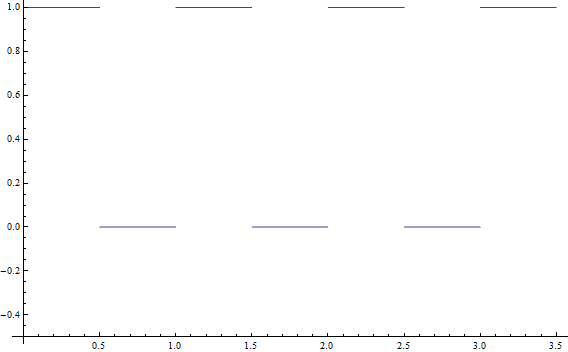
This function is the characteristic function of the set ${\cup }_{k\in \mathbb{Z}}[k,k+1/2]$. No matter how many terms we use, if the sum is finite then the result will be continuous, and this function is discontinuous. So we can’t represent it.

“Ah, what about continuous functions?” you say, “Surely if everything is continuous our problems will be solved.” Alas, if only mathematics were so simple. Here is an example of a continuous function which still cannot be represented: a triangle wave.

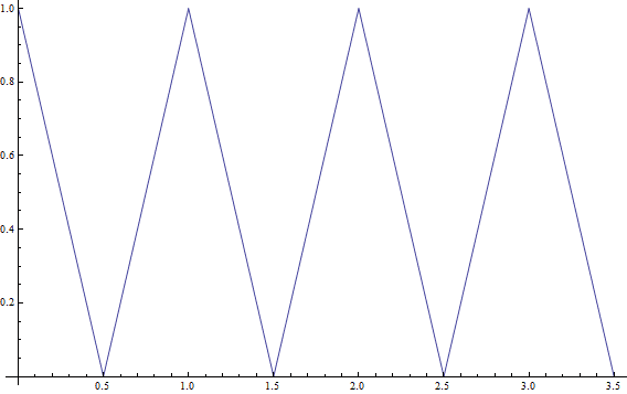
This function can be described as the periodization of the piecewise function defined by $1-2x$ and $2x$ on the intervals $[0,1/2],[1/2,1]$, respectively.

Unfortunately, these “sharp corners” prevent any finite sum from giving an exact representation. Indeed, this function is not differentiable at those points, while a finite sum of differentiable exponentials is.

More generally, this is a problem if the function we are trying to analyze is not smooth; that is, if it is not infinitely differentiable at all points in its domain. Since a complex exponential is smooth, and the sum of smooth functions is smooth, we see that this must be the case.

Indeed, the only way to avoid this issue is to let $n$ go to infinity. So let us make the natural definitions, and arrive at the true Fourier series:

Definition: The $k$-th Fourier coefficient of a function $f$, denoted $\hat{f}(k)$, is the integral

The Fourier series of $f$ is

and is equal to $f(t)$ for all $t\in \mathbb{R}$.

At first, we have to wonder what class of functions we can use this on. Indeed, this integral is not finite for some wild functions. This leads us to restrict Fourier series to functions in $L^2$. That is, the only functions we can apply this to must have finite $L^2$ norm. In the simplest terms, $f$ must be square-integrable, so that the integral

is finite. As it turns out, $L^2$ is a huge class of functions, and every function we might want to analyze in the real world is (or can be made to be) in $L^2$. Then, of course, the pointwise equality of a function with its Fourier series (pointwise convergence) is guaranteed by the fact that the complex exponentials form an orthonormal basis for $L^2$.

But we have other convergence concerns. Specifically, we want it to be the case that when $k$ is very far from 0, then $\hat{f}(k)$ contributes little to the representation of the function. The real way to say that this happens is by using the $L^2$ norm again, in the sense that two functions are “close” if the following integral is small in absolute value:

Indeed, if we let $g_n(t)$ be the termination of the Fourier series at $n$ (i.e. $-n\le k\le n$), then as $n\to \mathrm{\infty }$, the above integral tends to zero. This is called convergence in $L^2$, and it’s extremely important for applications. We will never be able to compute the true Fourier series in practice, so we have to stop at some sufficiently large $n$. We want the theoretical guarantee that our approximation only gets better for picking large $n$. The proof of this fact is again given by our basis: the complex exponentials form a complete basis with respect to the $L^2$ norm.

Moreover, if the original function $f$ is continuous then we get uniform convergence. That is, the quality of the approximation will not depend on $t$, but only on our choice of a terminating $n$.

There is a wealth of other results on the convergence of Fourier series, and rightly so, by how widely used they are. One particularly interesting result we note here is a counterexample: there are continuous and even integrable functions (but not square-integrable) for which the Fourier series diverges almost everywhere.

Other Bases, and an Application to Heat

As we said before, there is nothing special about using the complex exponentials as our orthonormal basis of $L^2$. More generally, we call $\left\{e_n\right\}$ a Hilbert basis for $L^2$ if it forms an orthonormal basis and is complete with respect to the $L^2$ norm.

One can define an analogous series expansion for a function with respect to any Hilbert basis. While we leave out many of the construction details for a later date, one can use, for example, Chebyshev polynomials or Hermite polynomials. This idea is hence generalized to the field of “wavelet analysis” and “wavelet transforms,” of which the Fourier variety is a special case (now we’re speaking quite roughly; there are details this author isn’t familiar with at the time of this writing).

Before we finish, we present an example where the Fourier series is used to solve the heat equation on a circular ring. We choose this problem because historically it was the motivating problem behind the development of these ideas.

In general, the heat equation applies to some region $R$ in space, and you start with an initial distribution of heat $f(x)$, where $x$ is a vector with the same dimension as $R$. The heat equation dictates how heat dissipates over time.

Periodicity enters into the discussion because of our region: $R$ is a one-dimensional circle, and so $x$ is just the value $x\in [0,1]$ parameterizing the angle $2\pi x$. Let $u(x,t)$ be the temperature at position $x$ at time $t$. As we just said, $u$ is 1-periodic in $x$, as is $f$. The two are related by $u(x,0)=f(x)$.

The important consideration is that the symmetry of the circle has consequences in how the heat dissipates.

Now let us write the Fourier series for $u$.

Where the dependence on time $t$ comes into play in $c_k$:

Now the mystery here is evaluating these $c_k$. We want to find the coefficients in terms of the initial temperature distribution $f$. The magical step here is that $u$ satisfies the (one-dimensional) heat equation: the partial derivative with respect to time of $u$ is directly proportional to the second partial spatial derivative. In symbols,

Where the constant $a$ depends on the physical properties of the region. See this page for a general derivation. This equation also called the diffusion equation, because it not only governs the dissipation of heat, but the diffusion of lots of quantities over time (e.g., charge in a wire).

Without loss of generality, let’s let $a=1/2$. Let’s plug the Fourier series for $u(x,t)$ into the heat equation and see what happens. First,

${\displaystyle u_t=\sum _{k=-\mathrm{\infty }}^{\mathrm{\infty }}{c}_k^{\prime }(t)e^{2\pi ikx}}$

And plugging in, we have

This simply says that we equate the coefficients of each term $e^{2\pi ikx}$, giving

But this is a wonderful thing, because this is an ordinary differential equation, and we can solve it by elementary means. Using the usual logarithmic trick, we have

So now $c_k(0)$ is just ${\int }_0^{1}u(x,0)e^{-2\pi ikx}dx$ and $u(x,0)=f(x)$. From a different perspective, this is just the $k$-th Fourier coefficient of $f$. Summing it all up, we now have a very explicit description of $u(x,t)$ in which the dependence on time and space is obvious:

And this solves the problem.

To convince you of some of the virtues of this representation, we can see that as $t$ tends to infinity, the first exponential goes to zero in every term, so that the whole expression goes to zero (regardless of $k,k^2$ is always positive). That is, no matter what the initial heat distribution is, after a long enough time all of the heat at any point will dissipate.

So there you have it! Our main content posts in the future will use Fourier series (and more heavily, Fourier transforms) in analyzing things like music files, images, and other digital quantities.

Until then!