The Discrete Fourier Transform — A Primer

So here we are. We have finally made it to a place where we can transition with confidence from the classical continuous Fourier transform to the discrete version, which is the foundation for applications of Fourier analysis to programming. Indeed, we are quite close to unfurling the might of the Fast Fourier Transform algorithm, which efficiently computes the discrete Fourier transform. But because of its focus on algorithmic techniques, we will save it for a main content post and instead focus here on the intuitive connections between the discrete and continuous realms.

The goal has roughly three parts:

1. Find a reasonable discrete approximation to a continuous function.
2. Find a reasonable discrete approximation to the Fourier transform of a continuous function.
3. Find a way to transition between the two discrete representations.

We should also note that there will be some notational clashes in the sequel. Rigorously, item 3 will result in an operation which we will denote by $ \mathscr{F}$, but will be distinct from the classical Fourier transform on continuous functions. Indeed, they will have algebraic similarities, but one operates on generalized functions, and the other on finite sequences. We will keep the distinction clear from context to avoid adding superfluous notation. Moreover, we will avoid the rigor from the last post on tempered distributions. Instead we simply assume all functions are understood to be distributions and use the classical notation. Again, this is safe because our dabbling with the classical transform will be solely for intuition.

Of course, the point of this entire post is that all of the facts we proved about the continuous Fourier transform have direct translations into the discrete case. Up to a constant factor (sometimes) and up to notational conventions, the two theories will be identical. This is part of the beauty of the subject; sit back and enjoy it.

Sampling

There is a very nice theorem about classical Fourier transforms that has to do with reconstructing a function from a discrete sample of its points. Since we do not actually need this theorem for anything other than motivation, we will not prove it here. Instead, we’ll introduce the definitions needed to state it, and see why it motivates a good definition for the discrete “approximation” to a function. For a much more thorough treatment of the sampling theorem and the other issues we glaze over in this post, see Chapter 5 of these lecture notes.

Definition: A function $ f$ is time limited if it has bounded support. A function $ f$ is bandlimited if its Fourier transform has bounded support. That is, if there is some $ B$ so that the Fourier transform of $ f$ is only nonzero when $ |s|bandwidth of $ f$.

To be honest, before seeing a mathematical treatment of signal processing, this author had no idea what bandwidth actually referred to. It’s nice to finally solve those life mysteries.

In any case, it often occurs that one has a signal $ f$ for which one can only measure values, but one doesn’t have access to an exact description of $ f$. The sampling theorem allows us to reconstruct $ f$ exactly by choosing certain sample points. In a simplified form, the theorem is as follows:

Theorem: Suppose $ f$ is a function of bandwidth $ B$. Then one can reconstruct $ f$ exactly from the set of points $ (k/2B, f(k/2B))$ as $ k$ ranges over $ \mathbb{Z}$ (that is, the sampling rate is at least $ 1/2B$).

Unsurprisingly, the proof uses the Fourier transform in a nontrivial way. Moreover, there is a similar theorem for the Fourier transform $ \mathscr{F}f$, which can be reconstructed exactly from its samples if the sampling rate is at least $ 1/L$, where $ L/2$ bounds the support of $ f$. Note that the sampling rate in one domain is determined by the limitations on the other domain.

What’s more, if we are daring enough to claim $ f$ is both time limited and bandlimited (and we sample as little as possible in each domain), then the number of sample points is the same for both domains. In particular, suppose $ f(t)$ is only nonzero on $ 0 \leq t \leq L$ and its Fourier transform on $ 0 \leq s \leq 2B$. Note that since $ f$ is both timelimited and bandlimited, there is no fault in shifting both so their smallest value is at the origin. Then, if $ n, m$ are the respective numbers of sampled points in the time and frequency domains, then $ m/L = 2B, n/2B = L$, and so $ m = n = 2BL$.

Now this gives us a good reason to define the discrete approximation to a signal as

$$\displaystyle f_{\textup{sampled}} = (f(t_0), f(t_1), \dots, f(t_{n-1})),$$

where $ t_k = k/2B$. This accomplishes our first task. Now, in order to determine what the discrete Fourier transform should look like, we can represent this discrete approximation as a distribution using shifted deltas:

$$\displaystyle f_{\textup{sampled}}(t) = \sum_{k=0}^{n-1}f(t_k)\delta(t-t_k)$$

Here the deltas ensure the function is zero at points not among the $ t_k$, capturing the essence of the finite sequence above. Taking the Fourier transform of this (recalling that the Fourier transform of the shifted delta is a complex exponential and using linearity), we get

$$\displaystyle \mathscr{F}f_{\textup{sampled}}(s) = \sum_{k=0}^{n-1}f(t_k)e^{-2 \pi i s t_k}$$

Denote the above function by $ F$. Now $ F$ is unfortunately still continuous, so we take the same approach we did for $ f$ and sample it via the samples in the frequency domain at $ s_j = j/L$. This gives the following list of values for the discrete approximation to the transformed version of $ f$:

$$\displaystyle F(s_0) = \sum_{k=0}^{n-1} f(t_k)e^{-2 \pi i s_0t_k}$$ $$\displaystyle F(s_1) = \sum_{k=0}^{n-1} f(t_k)e^{-2 \pi i s_1t_k}$$ $$\vdots$$ $$\displaystyle F(s_n) = \sum_{k=0}^{n-1} f(t_k)e^{-2 \pi i s_nt_k}$$

And now the rest falls together. We can denote by $ (\mathscr{F}f)_{\textup{sampled}}$ the tuple of values $ F(s_j)$, and the list of formulas above gives a way to transition from one domain to the other.

A Discrete Life

Now we move completely away from the continuous realm. The above discussion was nice in giving us an intuition for why the following definitions are reasonable. However, in order to actually use these ideas on discrete sequences, we can’t be restricted to sampling continuous functions. In fact, most of our planned work on this blog will not use discrete approximations to continuous functions, but just plain old sequences. So we just need to redefine the above ideas in a purely discrete realm.

The first step is to get rid of any idea of the sampling rate, and instead write everything in terms of the indices. This boils down to the a convenient coincidence. If $ t_k = k/2B, s_j = j/L$, then by our earlier remarks that $ 2BL = n$ (the number of sample points taken), then $ t_ks_j = kj/n$. This allows us to rewrite the complex exponentials as $ e^{-2 \pi i kj/n}$, which is entirely in terms of the number of points used and the indices of the summation.

In other words, we can finally boil all of this discussion down to the following definition. Before we get to it, we should note that we use the square bracket notation for lists. That is, if $ L$ is a list, then $ L[i]$ is the $ i$-th element of that list. Usually one would use subscripts to denote this, but we’d like to stay close to our notation for the continuous case, at least to make the parallels between the two theories more obvious.

Definition: Let $ f = (f[1], \dots f[n])$ be a vector in $ \mathbb{R}^n$. Then the discrete Fourier transform of $ f$ is defined by the vector $ (\mathscr{F}f[1], \dots, \mathscr{F}f[n])$, where

$$\displaystyle \mathscr{F}f[j] = \sum_{k=0}^{n-1} f[k]e^{-2 \pi i jk/n}$$

The phrase “discrete Fourier transform” is often abbreviated to DFT.

Now although we want to showcase the connections between the discrete and continuous Fourier transforms, we should note that they are completely disjoint. If one so desired (and many books follow this route) one could start with the discrete Fourier transform and later introduce the continuous version. We have the advantage of brevity here, in that we know what the theorems should say before we actually prove them. The point is that while the two transforms have connections and similarities, their theory is largely independent, and moreover the definition of the Fourier transform can be given without any preface. Much as we claimed with the continuous Fourier transform, the discrete Fourier transform is simply an operation on lists of data (i.e., on vectors).

Pushing the discrete to the extreme, we can represent the list of complex exponentials as a discrete signal too.

Definition: The discrete complex exponential of period $ n$ is the list

$$\displaystyle \omega_n = (1, e^{2 \pi i/n}, \dots, e^{2 \pi i (n-1)/n}).$$

We will omit the subscript $ n$ when it is understood (at least, for the rest of this primer). And hence $ \omega[k] = e^{2 \pi i k/n}$ and moreover $ \omega^m[k] = \omega^k[m] = e^{2\pi imk/n}$. If we denote by $ \omega^n$ the vector of entry-wise powers of $ \omega$, then we can write the discrete Fourier transform in its most succinct form as:

$$\displaystyle \mathscr{F}f[m] = \sum_{k=0}^{n-1} f[k]\omega^{-m}[k]$$

or, recognizing everything without indexing in “operator notation,”

$$\displaystyle \mathscr{F}f = \sum_{k=0}^{n-1}f\omega^{-m}.$$

There are other ways to represent the discrete Fourier transform as an operation. In fact, since we know the classical Fourier transform is a linear operator, we should be able to come up with a matrix representation of the discrete transform. We will do just this, and as a result we will find the inverse discrete Fourier transform, but first we should look at some examples.

The Transforms of Discrete Signals

Perhaps the simplest possible signal one could think of is the delta function, whose discretized form is

$$\displaystyle \delta = (1,0, \dots, 0)$$

with the corresponding shifted form

$$\displaystyle \delta_k = (0, 0, \dots 0, 1, 0, \dots 0)$$

where the 1 appears in the $ k$-th spot. The reader should be convinced that this is indeed the right definition because it’s continuous cousin’s defining properties translate nicely. Specifically, $ \sum_{k}\delta_m[k] f[k] = f[m]$ for all $ m$, and $ \sum_{k}\delta[k] = 1$.

Now to find its Fourier transform, we simply use the definition:

$$\displaystyle \mathscr{F}\delta[m] = \sum_{k=0}^{n-1}\delta[k] \omega^{-m}[k]$$

The only time that $ \delta[k]$ is nonzero is for $ k=0$, so this is simply the vector $ \delta[0] \omega^{0}$, which is the vector consisting entirely of 1’s. Hence, as in the continuous case (or at least, for the continuous definition of the 1 distribution),

$$\displaystyle \mathscr{F}\delta = 1$$

In an identical manner, one can prove that $ \mathscr{F}\delta_k = \omega^{-k}$, just as it was in for the continuous transform.

Now let’s do an example which deviates slightly from the continuous case. Recall that the continuous Fourier transform of the complex exponential was a delta function (to convince the reader, simply see that a single complex exponential can only have a single angular variable, and hence a singular frequency). In the discrete case, we get something similar.

\[ \displaystyle \mathscr{F}\omega^{d} = \sum_{k=0}^{n-1} \omega^d\omega^{-m}, \]

so looking at the $ m$-th entry of this vector, we get

$$\displaystyle \mathscr{F}\omega^d[m] = \sum_{k=0}^{n-1} \omega^d[k] \omega^{-m}[k]$$

but because $ \omega^{-m}[k] = e^{-2 \pi i km/n} = \overline{\omega^m[k]}$, we see that the sum is just the usual complex inner product $ \left \langle \omega^d, \omega^m \right \rangle$. Further, as the differing powers of $ \omega$ are orthogonal (hint: their complex inner product forms a geometric series), we see that they’re only nonzero when $ d =m$. In this case, it is easy to show that the inner product is precisely $ n$. Summarizing,

This is naturally $ n \delta_d$, so our final statement is just $ \mathscr{F}\omega^d = n\delta_d$. Note that here we have the extra factor of $ n$ floating around. The reason for this boils down to the fact that the norm of the complex exponential $ \omega$ is $ \sqrt{n}$, and not 1. That is, the powers of $ \omega$ do not form an orthonormal basis of $ \mathbb{C}^n$. There are various alternative definitions that try to compensate for this, but to the best of this author’s knowledge a factor of $ n$ always shows up in some of the resulting formulas. In other words, we should just accept this deviation from the continuous theory as collateral damage.

The mischievous presence of $ n$ also shows up in an interesting way in the inverse discrete Fourier transform.

The DFT and its Inverse, as a Matrix

It’s a trivial exercise to check by hand that the discrete Fourier transform is a linear operation on vectors. i.e., $ \mathscr{F}(v_1 + v_2)[m] = \mathscr{F}v_1[m] + \mathscr{F}v_2[m]$ for all vectors $ v_1, v_2$ and all $ m$. As we know from our primer on linear algebra, all such mappings are expressible as matrix multiplication by a fixed matrix.

The “compact” form we represented the discrete Fourier transform above sheds light onto this question. Specifically, the formula

$$\displaystyle \mathscr{F}f[m] = \sum_{k=0}^{n-1}f[k]\omega^{-m}[k]$$

Is basically just the definition of a matrix multiplication. Viewing $ f$ as the column vector

$$\displaystyle \begin{pmatrix} f[0]\\\ f[1]\\\ \vdots\\\ f[n] \end{pmatrix}$$

It is easy to see that the correct matrix to act on this vector is

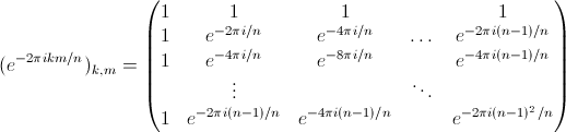
A perhaps easier way to digest this matrix is by viewing each row of the matrix as the vector $ \omega^{-m}$.

\[ \displaystyle \mathscr{F} = \begin{pmatrix} \textbf{—} & \omega^0 & \textbf{—} \\\ \textbf{—} & \omega^{-1} & \textbf{—} \\\ & \vdots & \\\ \textbf{—} & \omega^{-(n-1)} & \textbf{—} \end{pmatrix}$ \]

Now let’s just admire this matrix for a moment. What started many primers ago as a calculus computation requiring infinite integrals and sometimes divergent answers is now trivial to compute. This is our first peek into how to compute discrete Fourier transforms in a program, but unfortunately we are well aware of the fact that computing this naively requires $ O(n^2)$ computations. Our future post on the Fast Fourier Transform algorithm will take advantage of the structure of this matrix to improve this by an order or magnitude to $ O(n \log n)$.

But for now, let’s find the inverse Fourier transform as a matrix. From the first of the two matrices above, it is easy to see that the matrix for $ \mathscr{F}$ is symmetric. Indeed, the roles of $ k,m$ are identical in $ e^{-2\pi i km/n}$. Furthermore, looking at the second matrix, we see that $ \mathscr{F}$ is almost unitary. Recall that a matrix $ A$ is unitary if $ AA^* = I$, where $ I$ is the identity matrix and $ A^*$ is the conjugate transpose of $ A$. For the case of $ \mathscr{F}$, we have that $ \mathscr{FF^*} = nI$. We encourage the reader to work this out by hand, noting that each entry in the matrix resulting from $ \mathscr{FF^*}$ is an inner product of powers of $ \omega$.

In other words, we have $ \mathscr{F}\cdot \frac{1}{n}\mathscr{F^*} = I$, so that $ \mathscr{F}^{-1} = \frac{1}{n}\mathscr{F^*}$. Since $ \mathscr{F}$ is symmetric, this simplifies to $ \frac{1}{n}\overline{\mathscr{F}}$.

Expanding this out to a summation, we get what we might have guessed was the inverse transform:

$ \displaystyle \mathscr{F}^{-1}f[m] = \frac{1}{n} \sum_{k=0}^{n-1} f[k]\omega^m[k]$.

The only difference between this formula and our intuition is the factor of $ 1/n$.

Duality

The last thing we’d like to mention in this primer is that the wonderful results on duality for the continuous Fourier transform translate to the discrete (again, with a factor of $ n$). While we leave the details as an exercise to the reader,

In order to do this, we need some additional notation. We can think of $ \omega$ as an infinite sequence which would repeat itself every $ n$ entries (by Euler’s identity). Then we can “index” $ \omega$ higher than $ n$, and get the identity $ \omega^m[k] = \omega[mk]$. Similarly, we could “periodize” a discrete signal $ f$ so that $ f[m]$ is defined by $ f[m \mod n]$ and we allow $ m \in \mathbb{Z}$.

This periodization allows us to define $ f^-$ naturally as $ f^-[m] = f[-m \mod n]$. Then it becomes straightforward to check that $ \mathscr{F}f^- = (\mathscr{F}f)^-$, and as a corollary $ \mathscr{FF}f = nf^-$. This recovers some of our most powerful tools from the classical case for computing Fourier transforms of specific functions.

Next time (and this has been a long time coming) we’ll finally get to the computational meat of Fourier analysis. We’ll derive and implement the Fast Fourier Transform algorithm, which computes the discrete Fourier transform efficiently. Then we’ll take our first foray into playing with real signals, and move on to higher-dimensional transforms for image analysis.

Until then!

---

---