It’s often said that the Age of Information began on August 17, 1964 with the publication of Cooley and Tukey’s paper, “An Algorithm for the Machine Calculation of Complex Fourier Series.” They published a landmark algorithm which has since been called the Fast Fourier Transform algorithm, and has spawned countless variations. Specifically, it improved the best known computational bound on the discrete Fourier transform from $ O(n^2)$ to $ O(n \log n)$, which is the difference between uselessness and panacea.
Indeed, their work was revolutionary because so much of our current daily lives depends on efficient signal processing. Digital audio and video, graphics, mobile phones, radar and sonar, satellite transmissions, weather forecasting, economics and medicine all use the Fast Fourier Transform algorithm in a crucial way. (Not to mention that electronic circuits wouldn’t exist without Fourier analysis in general.) Before the Fast Fourier Transform algorithm was public knowledge, it simply wasn’t feasible to process digital signals.
Amusingly, Cooley and Tukey’s particular algorithm was known to Gauss around 1800 in a slightly different context; he simply didn’t find it interesting enough to publish, even though it predated the earliest work on Fourier analysis by Joseph Fourier himself.
In this post we will derive and implement a Fast Fourier Transform algorithm, and explore a (perhaps naive) application to audio processing. In particular, we will remove white noise from a sound clip by filtering the frequency spectrum of a noisy signal.
As usual, all of the resources used for this post are available on this blog’s Github page.
Derivation
It turns out that there are a number of different ways to speed up the naive Fourier Transform computation. As we saw in our primer on the discrete Fourier transform, the transform itself can be represented as a matrix. With a bit of nontrivial analysis, one can factor the Fourier transform matrix into a product of two sparse matrices (i.e., which contain mostly zeros), and from there the operations one can skip are evident. The intuitive reason why this should work is that the Fourier transform matrix is very structured, and the complex exponential has many useful properties. For more information on this method, see these lecture notes (p. 286).
We will take a different route which historically precedes the matrix factorization method. In fact, the derivation we’ll trace through below was Cooley and Tukey’s original algorithm. The method itself is a classical instance of a divide and conquer algorithm. Familiar programmers would recognize the ideas in common sorting algorithms: both mergesort and quicksort are divide and conquer algorithms.
The difficulty here is to split a list of numbers into two lists which are half in size in such a way that the Fourier transforms of the smaller pieces can be quickly combined to form the Fourier transform of the original list. Once we accomplish that, the rest of the algorithm falls out from recursion; further splitting each piece into two smaller pieces, we will eventually reach lists of length two or one (in which case the Fourier transform is completely trivial).
For now, we’ll assume that the length of the list is a power of 2. That is,
$ f = (f[1], f[2], \dots, f[n]), n = 2^k$ for some $ k$.
We will also introduce the somewhat helpful notation for complex exponentials. Specifically, $ \omega[p,q] = e^{2\pi i q/p}$. Here the $ p$ will represent the length of the list, and $ q$ will be related to the index. In particular, the complex exponential that usually shows up in the discrete Fourier transform (again, refer to our primer) is $ \omega[n, -km] = e^{-2 \pi i mk/n}$. We write the discrete Fourier transform of $ f$ by specifying its $ m$-th entry:
$$\displaystyle \mathscr{F}f[m] = \sum_{k=0}^{n-1} f[k]\omega[n, -km]$$Now the trick here is to split up the sum into two lists each of half size. Of course, one could split it up in many different ways, but after we split it we need to be able to rewrite the pieces as discrete Fourier transforms themselves. It turns out that if we split it into the terms with even indices and the terms with odd indices, things work out nicely.
Specifically, we can write the sum above as the two sums below. The reader should study this for a moment (or better yet, try to figure out what it should be without looking) to ensure that the indices all line up. The notation grows thicker ahead, so it’s good practice.
$ \displaystyle \mathscr{F}f[m] = \sum_{k=0}^{\frac{n}{2} – 1} f[2k] \omega[n,-2km] + \sum_{k=0}^{\frac{n}{2} – 1} f[2k+1]\omega[n,-(2k+1)m]$.
Now we need to rewrite these pieces as Fourier transforms. Indeed, we must replace the occurrences of $ n$ in the complex exponentials with $ n/2$. This is straightforward in the first summation, since
$ \omega[n, -2km] = e^{-2 \pi i km/n} = \omega[\frac{n}{2}, -km]$.
For the second summation, we observe that
$ \displaystyle \omega[n, -(2k+1)m] = \omega[n, -2km] \cdot \omega[n,-m]$.
Now if we factor out the $ \omega[n,-m]$, we can transform the second sum in the same way as the first, but with that additional factor out front. In other words, we now have
$ \displaystyle \mathscr{F}f[m] = \sum_{k=0}^{\frac{n}{2}-1} f[2k] \omega[n/2, -km] + \omega[n, -m] \sum_{k=0}^{\frac{n}{2}-1}f[2k+1] \omega[n/2, -km]$.
If we denote the list of even-indexed entries of $ f$ by $ f_{\textup{even}}$, and vice versa for $ f_{\textup{odd}}$, we see that this is just a combination of two Fourier transforms of length $ n/2$. That is,
$$\displaystyle \mathscr{F}f = \mathscr{F}f_{\textup{even}} + \omega[n,-m] \mathscr{F}f_{\textup{odd}}$$But we have a big problem here. Computer scientists will recognize this as a type error. The thing on the left hand side of the equation is a list of length $ n$, while the thing on the right hand side is a sum of two lists of length $ n/2$, and so it has length $ n/2$. Certainly it is still true for values of $ m$ which are less than $ n/2$; we broke no algebraic laws in the way we rewrote the sum (just in the use of the $ \mathscr{F}$ notation).
Recalling our primer on the discrete Fourier transform, we naturally extended the signals involved to be periodic. So indeed, the length-$ n/2$ Fourier transforms satisfy the following identity for each $ m$.
$$\mathscr{F}f_{\textup{even}}[m] = \mathscr{F}f_{\textup{even}}[m+n/2] \\\ \mathscr{F}f_{\textup{odd}}[m] = \mathscr{F}f_{\textup{odd}}[m+n/2]$$However, this does not mean we can use the same formula above! Indeed, for a length $ n$ Fourier transform, it is not true in general that $ \mathscr{F}f[m] = \mathscr{F}f[m+n/2]$. But the correct formula is close to it. Plugging in $ m + n/2$ to the summations above, we have
$$\displaystyle \mathscr{F}f[m+n/2] = \sum_{k=0}^{\frac{n}{2} – 1}f[2k] \omega[n/2, -(m+n/2)k] + \\\ \omega[n, -(m+n/2)] \sum_{k=0}^{\frac{n}{2} – 1}f[2k+1] \omega[n/2, -(m+n/2)k]$$Now we can use the easy-to-prove identity
$$\displaystyle \omega[n/2, -(m+n/2)k] = \omega[n/2, -mk] \omega[n/2, -kn/2]$$And see that the right-hand-term is simply $ e^{2 \pi i k} = 1$. Similarly, one can trivially prove the identity
$ \displaystyle \omega[n, -(m+n/2)] = \omega[n, -m] \omega[n, -n/2] = -\omega[n, -m]$,
this simplifying the massive formula above to the more familiar
$$\displaystyle \mathscr{F}f[m + n/2] = \sum_k f[2k]\omega[n/2, -mk] – \omega[n, -m] \sum_k f[2k+1] \omega[n/2, -mk]$$Now finally, we have the Fast Fourier Transform algorithm expressed recursively as:
$ \displaystyle \mathscr{F}f[m] = \mathscr{F}f_{\textup{even}}[m] + \omega[n,-m] \mathscr{F}f_{\textup{odd}}[m]$
$$\displaystyle \mathscr{F}f[m+n/2] = \mathscr{F}f_{\textup{even}}[m] – \omega[n,-m] \mathscr{F}f_{\textup{odd}}[m]$$With the base case being $ \mathscr{F}([a]) = [a]$.
In Python
With all of that notation out of the way, the implementation is quite short. First, we should mention a few details about complex numbers in Python. Much to this author’s chagrin, Python represents $ i$ using the symbol 1j. That is, in python, $ a + bi$ is
a + b * 1j
Further, Python reserves a special library for complex numbers, the cmath library. So we implement the omega function above as follows.
import cmath

def omega(p, q):
   return cmath.exp((2.0 * cmath.pi * 1j * q) / p)
And then the Fast Fourier Transform algorithm is more or less a straightforward translation of the mathematics above:
def fft(signal):
   n = len(signal)
   if n == 1:
      return signal
   else:
      Feven = fft([signal[i] for i in xrange(0, n, 2)])
      Fodd = fft([signal[i] for i in xrange(1, n, 2)])

      combined = [0] * n
      for m in xrange(n/2):
         combined[m] = Feven[m] + omega(n, -m) * Fodd[m]
         combined[m + n/2] = Feven[m] - omega(n, -m) * Fodd[m]

      return combined
Here I use the awkward variable names “Feven” and “Fodd” to be consistent with the notation above. Note that this implementation is highly non-optimized. There are many ways to improve the code, most notably using a different language and cacheing the complex exponential computations. In any event, the above code is quite readable, and a capable programmer could easily speed this up by orders of magnitude.
Of course, we should test this function on at least some of the discrete signals we investigated in our primer. And indeed, it functions correctly on the unshifted delta signal
>>> fft([1,0,0,0])
[(1+0j), (1+0j), (1+0j), (1+0j)]
>>> fft([1,0,0,0,0,0,0,0])
[(1+0j), (1+0j), (1+0j), (1+0j), (1+0j), (1+0j), (1+0j), (1+0j)]
As well as the shifted verion (up to floating point roundoff error)
>>> fft([0,1,0,0])
[(1+0j),
 (6.123233995736766e-17-1j),
 (-1+0j),
 (-6.123233995736766e-17+1j)]
>>> fft([0,1,0,0,0,0,0,0])
[(1+0j),
 (0.7071067811865476-0.7071067811865475j),
 (6.123233995736766e-17-1j),
 (-0.7071067811865475-0.7071067811865476j),
 (-1+0j),
 (-0.7071067811865476+0.7071067811865475j),
 (-6.123233995736766e-17+1j),
 (0.7071067811865475+0.7071067811865476j)]
And testing it on various other shifts gives further correct outputs. Finally, we test the Fourier transform of the discrete complex exponential, which the reader will recall is a scaled delta.
>>> w = cmath.exp(2 * cmath.pi * 1j / 8)
>>> w
(0.7071067811865476+0.7071067811865475j)
>>> d = 4
>>> fft([w**(k*d) for k in range(8)])
[                           1.7763568394002505e-15j,
 (-7.357910944937894e-16  + 1.7763568394002503e-15j),
 (-1.7763568394002505e-15 + 1.7763568394002503e-15j),
 (-4.28850477329429e-15   + 1.7763568394002499e-15j),
 (8                       - 1.2434497875801753e-14j),
 (4.28850477329429e-15    + 1.7763568394002505e-15j),
 (1.7763568394002505e-15  + 1.7763568394002505e-15j),
 (7.357910944937894e-16   + 1.7763568394002505e-15j)]
Note that $ n = 8$ occurs in the position with index $ d=4$, and all of the other values are negligibly close to zero, as expected.
So that’s great! It works! Unfortunately it’s not quite there in terms of usability. In particular, we require our signal to have length a power of two, and most signals don’t happen to be that long. It turns out that this is a highly nontrivial issue, and all implementations of a discrete Fourier transform algorithm have to compensate for it in some way.
The easiest solution is to simply add zeros to the end of the signal until it is long enough, and just work with everything in powers of two. This technique (called zero-padding) is only reasonable if the signal in question is actually zero outside of the range it’s sampled from. Otherwise, subtle and important things can happen. We’ll leave further investigations to the reader, but the gist of the idea is that the Fourier transform assumes periodicity of the data one gives it, and so padding with zeros imposes a kind of periodicity that is simply nonexistent in the actual signal.
Now, of course not every Fast Fourier transform uses zero-padding. Unfortunately the techniques to evaluate a non-power-of-two Fourier transform are relatively complex, and beyond the scope of this post (though not beyond the scope of this blog). The interested reader should investigate the so-called Chirp Z-transform, as discovered by Rader, et al. in 1968. We may cover it here in the future.
In any case, the code above is a good starting point for any technique, and as usual it is available on this blog’s Github page. Finally, the inverse transform has a simple implementation, since it can be represented in terms of the forward transform (hint: remember duality!). We leave the code as an exercise to the reader.
Experiments with Sound — I am no Tree!

For the remainder of this post we’ll use a more established Fast Fourier Transform algorithm from the Python numpy library. The reasons for this are essentially convenience. Being implemented in C and brandishing the full might of the literature on Fourier transform algorithms, the numpy implementation is lightning fast. Now, note that the algorithm we implemented above is still correct (if one uses zero padding)! The skeptical reader may run the code to verify this. So we are justified in abandoning our implementation until we decide to seriously focus on improving its speed.
So let’s play with sound.
The sound clip we’ll be using is the following piece of dialog from the movie The Lord of the Rings: The Two Towers. We include the original wav file with the code on this blog’s Github page.
If we take the Fourier transform of the sound sample, we get the following plot of the frequency spectrum. Recall, the frequency spectrum is the graph of the norm of the frequency values.
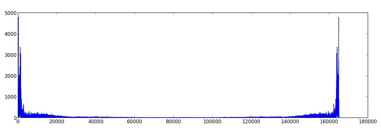
Here we note that there is a symmetry to the graph. This is not a coincidence: if the input signal is real-valued, it will always be the case that the Fourier transform is symmetric about its center value. The reason for this goes back to our first primer on the Fourier series, in that the negative coefficients were complex conjugates of the positive ones. In any event, we only need concern ourselves with the first half of the values.
We will omit the details for doing file I/O with audio. The interested reader can inspect our source code, and they will find a very basic use of the scikits.audiolab library, and matplotlib for plotting the frequency spectrum.
Now, just for fun, let’s tinker with this audio bite. First we’ll generate some random noise in the signal. That is, let’s mutate the input signal as follows:
import random
inputSignal = [x/2.0 + random.random()*0.1 for x in inputSignal]
This gives us a sound bite with an annoying fuzziness in the background:
Next, we will use the Fourier transform to remove some of this noise. Of course, since the noise is random it inhabits all the frequencies to some degree, so we can’t eliminate it entirely. Furthermore, as the original audio clip uses some of the higher frequencies, we will necessarily lose some information in the process. But in the real world we don’t have access to the original signal, so we should clean it up as best we can without losing too much information.
To do so, we can plot the frequencies for the noisy signal:
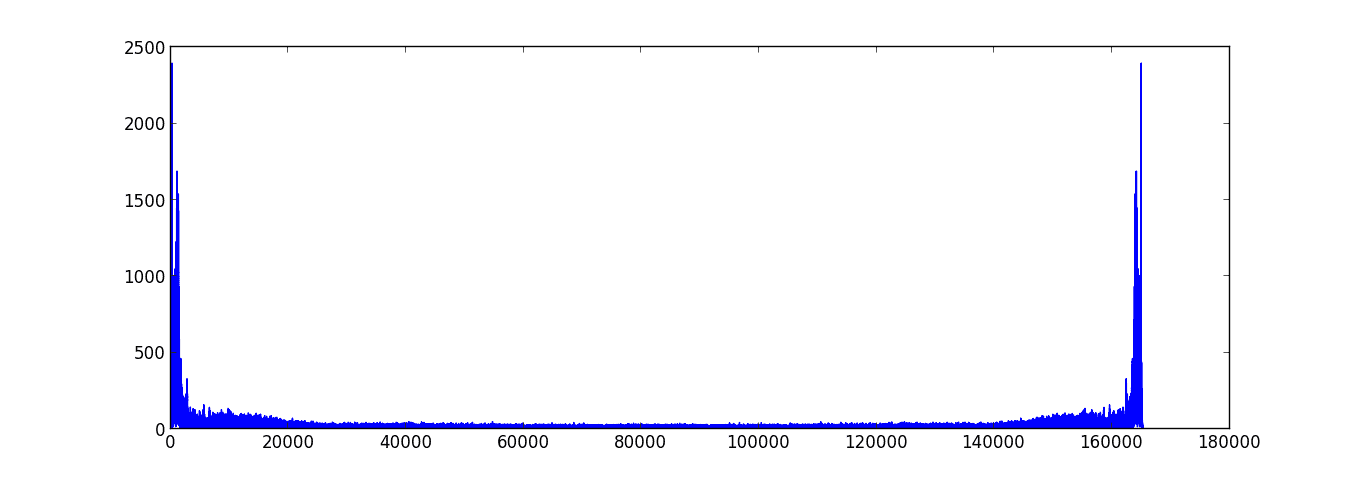
Comparing this with our original graph (cheating, yes, but the alternative is to guess and check until we arrive at the same answer), we see that the noise begins to dominate the spectrum at around the 20,000th index. So, we’ll just zero out all of those frequencies.
def frequencyFilter(signal):
   for i in range(20000, len(signal)-20000):
      signal[i] = 0
And voila! The resulting audio clip, while admittedly damaged, has only a small trace of noise:
Inspecting the source code, one should note that at one point we halve the amplitude of the input signal (i.e., in the time domain). The reason for this is if one arbitrarily tinkers with the frequencies of the Fourier transform, it can alter the amplitude of the original signal. As one quickly discovers, playing the resulting signal as a wav file can create an unpleasant crackling noise. The amplitudes are clipped (or wrapped around) by the audio software or hardware for a reason which is entirely mysterious to this author.
In any case, this is clearly not the optimal way (or even a good way) to reduce white noise in a signal. There are certainly better methods, but for the sake of time we will save them for future posts. The point is that we were able to implement and use the Fast Fourier Transform algorithm to analyze the discrete Fourier transform of a real-world signal, and manipulate it in logical ways. That’s quite the milestone considering where we began!
Next up in this series we’ll investigate more techniques on sound processing and other one-dimensional signals, and we’ll also derive a multi-dimensional Fourier transform so that we can start working with images and other two-dimensional signals.
Until then!
Want to respond? Send me an email, post a webmention, or find me elsewhere on the internet.