The Cellular Automaton Method for Cave Generation

Dear reader, this post has an interactive simulation! We encourage you to play with it as you read the article below.

In our series of posts on cellular automata, we explored Conway’s classic Game of Life and discovered some interesting patterns therein. And then in our primers on computing theory, we built up a theoretical foundation for similar kinds of machines, including a discussion of Turing machines and the various computational complexity classes surrounding them. But cellular automata served us pretty exclusively as a toy. It was a basic model of computation, which we were interested in only for its theoretical universality. One wouldn’t expect too many immediately practical (and efficient) applications of something which needs a ridiculous scale to perform basic logic. In fact, it’s amazing that there are as many as there are.

In this post we’ll look at one particular application of cellular automata to procedural level generation in games.

The Need for More Caves

Level design in video games is a time-consuming and difficult task. It’s extremely difficult for humans to hand-craft areas that both look natural and are simultaneously fun to play in. This is particularly true of the multitude of contemporary role-playing games modeled after Dungeons and Dragons, in which players move through a series of areas defeating enemies, collecting items, and developing their character. With a high demand for such games and so many levels in each game, it would save an unfathomable amount of money to have computers generate the levels on the fly. Perhaps more importantly, a game with randomly generated levels inherently has a much higher replay value.

The idea of randomized content generation (often called procedural generation) is not particularly new. It has been around at least since the 1980’s. Back then, computers simply didn’t have enough space to store large, complex levels in memory. To circumvent this problem, video game designers simply generated the world as the player moved through it. This opened up an infinitude of possible worlds for the user to play in, and the seminal example of this is a game called Rogue, which has since inspired series such as Diablo, Dwarf Fortress, and many many others. The techniques used to design these levels have since been refined and expanded into a toolbox of techniques which have become ubiquitous in computer graphics and game development.

We’ll explore more of these techniques in the future, but for now we’ll see how a cellular automaton can be used to procedurally generate two-dimensional cave-like maps.

A Quick Review of Cellular Automata

While the interested reader can read more about cellular automata on this blog, we will give a quick refresher here.

For our purposes here, a 2-dimensional cellular automaton is a grid of cells $ G$, where each cell $ c \in G$ is in one of a fixed number of states, and has a pre-determined and fixed set of neighbors. Then $ G$ is updated by applying a fixed rule to each cell simultaneously, and the process is repeated until something interesting happens or boredom strikes the observer. The most common kind of cellular automaton, called a ‘Life-like automaton,’ has only two states, ‘dead’ and ‘alive’ (for us, 0 and 1), and the rule applied to each cell is given as conditions to be ‘born’ or ‘survive’ based on the number of adjacent live cells. This is often denoted “Bx/Sy” where x and y are lists of single digit numbers. Furthermore, the choice of neighborhood is the eight nearest cells (i.e., including the diagonally-adjacent ones). For instance, B3/S23 is the cellular automaton rule where a cell is born if it has three living neighbors, and it survives if it has either two or three living neighbors, and dies otherwise. Technically, these are called ‘Life-like automata,’ because they are modest generalizations of Conway’s original Game of Life. We give an example of a B3/S23 cellular automaton initialized by a finite grid of randomly populated cells below. Note that each of the black (live) cells in the resulting stationary objects satisfy the S23 part of the rule, but none of the neighboring white (dead) cells satisfy the B3 condition.

A cellular automaton should really be defined for an arbitrary graph (or more generally, an arbitrary state space). There is really nothing special about a grid other than that it’s easy to visualize. Indeed, some cellular automata are designed for hexagonal grids, others are embedded on a torus, and still others are one- or three-dimensional. Of course, nothing stops automata from existing in arbitrary dimension, or from operating with arbitrary (albeit deterministic) rules, but to avoid pedantry we won’t delve into a general definition here. It would take us into a discussion of discrete dynamical systems (of which there are many, often with interesting pictures).

It All Boils Down to a Simple Rule

Now the particular cellular automaton we will use for cave generation is simply B678/S345678, applied to a random initial grid with a fixed live border. We interpret the live cells as walls, and the dead cells as open space. This rule should intuitively work: walls will stay walls even if more cells are born nearby, but isolated or near-isolated cells will often be removed. In other words, this cellular automaton should ‘smooth out’ a grid arrangement to some extent. Here is an example animation quickly sketched up in Mathematica to witness the automaton in action:

As usual, the code to generate this animation (which is only a slight alteration to the code used in our post on cellular automata) is available on this blog’s Github page.

This map is already pretty great! It has a number of large open caverns, and they are connected by relatively small passageways. With a bit of imagination, it looks absolutely cavelike!

We should immediately note that there is no guarantee that the resulting regions of whitespace will be connected. We got lucky with this animation, in that there are only two disconnected components, and one is quite small. But in fact one can be left with multiple large caves which have no connecting paths.

Furthermore, we should note the automaton’s rapid convergence to a stable state. Unlike Conway’s Game of Life, in practice this automaton almost always converges within 15 steps, and this author has yet to see any oscillatory patterns. Indeed, they are unlikely to exist because the survival rate is so high, and our initial grid has an even proportion of live and dead cells. There is no overpopulation that causes cells to die off, so once a cell is born it will always survive. The only cells that do not survive are those that begin isolated. In a sense, B678/S345678 is designed to prune the sparse areas of the grid, and fill in the dense areas by patching up holes.

We should also note that the initial proportion of cells which are alive has a strong effect on the density of the resulting picture. For the animation we displayed above, we initially chose that 45% of the cells would be live. If we increase that a mere 5%, we get a picture like the following.

As expected, there are many more disconnected caverns. Some game designers prefer a denser grid combined with heuristic methods to connect the caverns. Since our goal is just to explore the mathematical ideas, we will leave this as a parameter in our final program.

Javascript Implementation, and Greater Resolution

One important thing to note is that B678/S345678 doesn’t scale well to fine grid sizes. For instance, if we increase the grid size to 200×200, we get something resembling an awkward camouflage pattern.

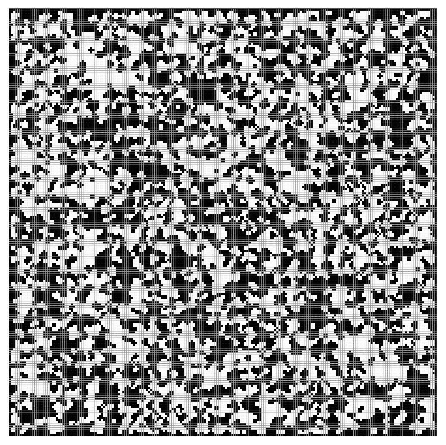
What we really want is a way to achieve the major features of the low-resolution image on a larger grid. Since cellular automata are inherently local manipulations, we should not expect any modification of B678/S345678 to do this for us. Instead, we will use B678/345678 to create a low-resolution image, increase its resolution manually, and smooth it out with — you guessed it — another cellular automaton! We’ll design this automaton specifically for the purpose of smoothing out corners.

To increase the resolution, we may simply divide the cells into four pieces. The picture doesn’t change, but the total number of cells increases fourfold. There are a few ways to do this programmatically, but the way we chose simply uses the smallest resolution possible, and simulates higher resolution by doing block computations. The interested programmer can view our Javascript program available on this blog’s Github page to see this directly (or view the page source of this post’s interactive simulator).

To design a “smoothing automaton,” we should investigate more closely what we need to improve on in the above examples. In particular, once we increase the resolution, we will have a lot of undesirable convex and concave corners. Since a “corner” is simply a block satisfying certain local properties, we can single those out to be removed by an automaton. It’s easy to see that convex corners have exactly 3 live neighbors, so we should not allow those cells to survive. Similarly, the white cell just outside a concave corner has 5 live neighbors, so we should allow that cell to be born. On the other hand, we still want the major properties of our old B678/S345678 to still apply, so we can simply add 5 to the B part and remove 3 from the S part. Lastly, for empirical reasons, we also decide to kill off cells with 4 live neighbors.

And so our final “smoothing automaton” is simply B5678/S5678.

We present this application as an interactive javascript program. Some basic instructions:

• The “Apply B678/S345678” button does what you’d expect: it applies B678/S345678 to the currently displayed grid. It iterates the automaton 20 times in an animation.
• The “Apply B5678/S5678” button applies the smoothing automaton, but it does so only once, allowing the user to control the degree of smoothing at the specific resolution level.
• The “Increase Resolution” button splits each cell into four, and may be applied until the cell size is down to a single pixel.
• The “Reset” button resets the entire application, creating a new random grid.

We used this program to generate a few interesting looking pictures by varying the order in which we pressed the various buttons (it sounds silly, but it’s an exploration!). First, a nice cave:

We note that this is not perfect. There are some obvious and awkward geometric artifacts lingering in this map, mostly in the form of awkwardly straight diagonal lines and awkwardly flawless circles. Perhaps one might imagine the circles are the bases of stalactites or stalagmites. But on the whole, in terms of keeping the major features of the original automaton present while smoothing out corners, this author thinks B5678/S5678 has done a phenomenal job. Further to the cellular automaton’s defense, when the local properties are applied uniformly across the entire grid, such regularities are bound to occur. That’s just another statement of the non-chaotic nature of B5678/S5678 (in stark contrast to Conway’s Game of Life).

There are various modifications one could perform (or choose not to, depending on the type of game) to make the result more accessible for the player. For instance, one could remove all regions which fit inside a sufficiently small circle, or add connections between the disconnected components at some level of resolution. This would require some sort of connected-component labeling, which is a nontrivial task; current research goes into optimizing connected-component algorithms for large-scale grids. We plan to cover such topics on this blog in the future.

Another example of a cool picture we created with this application might be considered a more “retro” style of cave.

We encourage the reader to play around with the program to see what other sorts of creations one can make. As of the time of this writing, changing the initial proportion of live cells (50%) or changing the automaton rules cannot be done in the browser; it requires one to modify the source code. We may implement the ability to control these in the browser given popular demand, but (of course) it would be a wonderful exercise for the intermediate Javascript programmer.

Caves in Three Dimensions

It’s clear that this same method can be extended to a three-dimensional model for generating caverns in a game like Minecraft. While we haven’t personally experimented with three-dimensional cellular automata here on this blog, it’s far from a new idea. Once we reach graphics programming on this blog (think: distant future) we plan to revisit the topic and see what we can do.

Until then!