The Recipe for Classification
One important task in machine learning is to classify data into one of a fixed number of classes. For instance, one might want to discriminate between useful email and unsolicited spam. Or one might wish to determine the species of a beetle based on its physical attributes, such as weight, color, and mandible length. These “attributes” are often called “features” in the world of machine learning, and they often correspond to dimensions when interpreted in the framework of linear algebra. As an interesting warm-up question for the reader, what would be the features for an email message? There are certainly many correct answers.
The typical way of having a program classify things goes by the name of supervised learning. Specifically, we provide a set of already-classified data as input to a training algorithm, the training algorithm produces an internal representation of the problem (a model, as statisticians like to say), and a separate classification algorithm uses that internal representation to classify new data. The training phase is usually complex and the classification algorithm simple, although that won’t be true for the method we explore in this post.
More often than not, the input data for the training algorithm are converted in some reasonable way to a numerical representation. This is not as easy as it sounds. We’ll investigate one pitfall of the conversion process in this post, but in doing this we separate the data from the application domain in a way that permits mathematical analysis. We may focus our questions on the data and not on the problem. Indeed, this is the basic recipe of applied mathematics: extract from a problem the essence of the question you wish to answer, answer the question in the pure world of mathematics, and then interpret the results.
We’ve investigated data-oriented questions on this blog before, such as, “is the data linearly separable?” In our post on the perceptron algorithm, we derived an algorithm for finding a line which separates all of the points in one class from the points in the other, assuming one exists. In this post, however, we make a different structural assumption. Namely, we assume that data points which are in the same class are also close together with respect to an appropriate metric. Since this is such a key point, it bears repetition and elevation in the typical mathematical fashion. The reader should note the following is not standard terminology, and it is simply a mathematical restatement of what we’ve already said.
The Axiom of Neighborliness: Let $ (X, d)$ be a metric space and let $ S \subset X$ be a finite set whose elements are classified by some function $ f : S \to \left \{ 1, 2, \dots, m \right \}$. We say that $ S$ satisfies the axiom of neighborliness if for every point $ x \in S$, if $ y$ is the closest point to $ x$, then $ f(x) = f(y)$. That is, $ y$ shares the same class as $ x$ if $ y$ is the nearest neighbor to $ x$.
For a more in-depth discussion of metrics, the reader should refer to this blog’s primer on the topic. For the purpose of this post and all foreseeable posts, $ X$ will always be $ \mathbb{R}^n$ for some $ n$, while the metric $ d$ will vary.
This axiom is actually a very strong assumption which is certainly not true of every data set. In particular, it highly depends on the problem setup. Having the wrong kinds or the wrong number of features, doing an improper conversion, or using the wrong metric can all invalidate the assumption even if the problem inherently has the needed structure. Luckily, for real-world applications we only need the data to adhere to the axiom of neighborliness in approximation (indeed, in practice the axiom is only verifiable in approximation). Of course, what we mean by “approximation” also depends on the problem and the user’s tolerance for error. Such is the nature of applied mathematics.
Once we understand the axiom, the machine learning “algorithm” is essentially obvious. For training, store a number of data points whose classes are known and fix a metric. To determine the class of an unknown data point, simply use the most common class of its nearest neighbors. As one may vary (as a global parameter) the number of neighbors one considers, this method is intuitively called k-nearest-neighbors.
The Most Basic Way to Learn: Copy Your Neighbors
Let’s iron out the details with a program and test it on some dummy data. Let’s construct a set of points in $ \mathbb{R}^2$ which manifestly satisfies the axiom of neighborliness. To do this, we’ll use Python’s random library to make a dataset sampled from two independent normal distributions.
import random

def gaussCluster(center, stdDev, count=50):
    return [(random.gauss(center[0], stdDev),
             random.gauss(center[1], stdDev)) for _ in range(count)]

def makeDummyData():
    return gaussCluster((-4,0), 1) + gaussCluster((4,0), 1)
The first function simply returns a cluster of points drawn from the specified normal distribution. For simplicity we equalize the covariance of the two random variables. The second function simply combines two clusters into a data set.
To give the dummy data class “labels,” we’ll simply have a second list that we keep alongside the data. The index of a data point in the first list corresponds to the index of its class label in the second. There are likely more elegant ways to organize this, but it suffices for now.
Implementing a metric is similarly straightforward. For now, we’ll use the standard Euclidean metric. That is, we simply take the sum of the squared differences of the coordinates of the given two points.
import math

def euclideanDistance(x,y):
    return math.sqrt(sum([(a-b)**2 for (a,b) in zip(x,y)]))
To actually implement the classifier, we create a function which itself returns a function.
import heapq

def makeKNNClassifier(data, labels, k, distance):
    def classify(x):
        closestPoints = heapq.nsmallest(k, enumerate(data),
                                        key=lambda y: distance(x, y[1]))
        closestLabels = [labels[i] for (i, pt) in closestPoints]
        return max(set(closestLabels), key=closestLabels.count)

    return classify
There are a few tricky things going on in this function that deserve discussion. First and foremost, we are defining a function within another function, and returning the created function. The important technical point here is that the created function retains all local variables which are in scope even after the function ends. Specifically, you can call “makeKNNClassifier” multiple times with different arguments, and the returned functions won’t interfere with each other. One is said to close over the values in the environment, and so this programming language feature is called a function closure or just a closure, for short. It allows us, for instance, to keep important data visible while hiding any low-level data it depends on, but which we don’t access directly. From a high level, the decision function entirely represents the logic of the program, and so this view is justified.
Second, we are using some relatively Pythonic constructions. The first line of “classify” uses of heapq to pick the $ k$ smallest elements of the data list, but in addition we use “enumerate” to preserve the index of the returned elements, and a custom key to have the judgement of “smallest” be determined by the custom distance function. Note that the indexed “y[1]” in the lambda function uses the point represented by “y” and not the saved index.
The second line simply extracts a list of the labels corresponding each of the closest points returned by the call to “nsmallest.” Finally, the third line returns the maximum of the given labels, where a label’s weight (determined by the poorly named “key” lambda) is its frequency in the “closestLabels” list.
Using these functions is quite simple:
trainingPoints = makeDummyData() # has 50 points from each class
trainingLabels = [1] * 50 + [2] * 50  # an arbitrary choice of labeling

f = makeKNNClassifier(trainingPoints, trainingLabels, 8, euclideanDistance)
print f((-3,0))
The reader may fiddle around with this example as desired, but we will not pursue it further. As usual, all code used in this post is available on this blog’s Github page. Let’s move on to something more difficult.
Handwritten Digits
One of the most classic examples in the classification literature is in recognizing handwritten digits. This originally showed up (as the legend goes) in the context of the United States Postal Service for the purpose of automatically sorting mail by the zip code of the destination. Although this author has no quantitative proof, the successful implementation of a scheme would likely save an enormous amount of labor and money. According to the Postal Facts site, there are 31,509 postal offices in the U.S. and, assuming each one processes mail, there is at least one employee at each office who would spend some time sorting by zip code. Given that the USPS processes 23 million pieces of mail per hour, a conservative estimate puts each office spending two hours of labor per day on sorting mail by zip code (resulting in a very rapid pace of 146.52 pieces of mail sorted per minute per worker). At a lower bound of $18/hr this amounts to a cost of $1,134,324 per day, or over 400 million dollars per year. Put in perspective, in one year the amount of money saved equals the entire two-year tuition of Moraine Valley Community College for 68,000 students (twice the current enrollment).
In short, the problem of sorting mail (and of classifying handwritten digits) begs to be automated, and indeed it has been to some degree for about four decades. Let’s see how k-nearest-neighbors fares in this realm.
We obtain our data from the UCI machine learning repository, and with a few minor modifications, we present it on this blog’s Github page (along with the rest of the code used in this post). A single line of the data file represents a handwritten digit and its label. The digit is a 256-element vector obtained by flattening a 16×16 binary-valued image in row-major order; the label is an integer representing the number in the picture. The data file contains 1593 instances with about 160 instances per digit.
In other words, our metric space is $ \left \{ 0,1 \right \}^{256}$, and we choose the Euclidean metric for simplicity. With the line wrapping to better display the “image,” one line from the data file looks like:
0 0 0 0 0 0 0 0 0 0 0 1 1 1 1 1
0 0 0 0 0 0 0 0 0 1 1 1 1 0 0 0
0 0 0 0 0 0 0 1 1 1 1 0 0 0 0 0
0 0 0 0 0 0 1 1 0 0 0 0 0 0 0 0
0 0 0 0 1 1 1 1 0 0 0 0 0 0 0 0
0 0 0 1 1 0 0 0 0 0 0 0 0 0 0 0
0 0 1 1 1 1 1 1 0 0 0 0 0 0 0 0
0 1 1 1 1 1 1 1 1 0 0 0 0 0 0 0
1 1 1 1 1 0 0 0 1 1 1 0 0 0 0 0
1 1 1 0 0 0 0 0 0 1 1 0 0 0 0 0
1 1 1 0 0 0 0 0 0 1 1 0 0 0 0 0
1 1 0 0 0 0 0 0 0 1 1 0 0 0 0 0
1 1 0 0 0 0 0 0 1 1 0 0 0 0 0 0
1 1 0 0 0 0 0 1 1 0 0 0 0 0 0 0
1 1 1 1 1 1 1 1 1 0 0 0 0 0 0 0
0 0 1 1 1 0 0 0 0 0 0 0 0 0 0 0, 6
After reading in the data appropriately, we randomly split the data set into two pieces, train on one piece, and test on the other. The following function does this, returning the success rate of the classification algorithm on the testing piece.
import knn
import random

def column(A, j):
   return [row[j] for row in A]

def test(data, k):
   random.shuffle(data)
   pts, labels = column(data, 0), column(data, 1)

   trainingData = pts[:800]
   trainingLabels = labels[:800]
   testData = pts[800:]
   testLabels = labels[800:]

   f = knn.makeKNNClassifier(trainingData, trainingLabels,
                             k, knn.euclideanDistance)
   correct = 0
   total = len(testLabels)

   for (point, label) in zip(testData, testLabels):
      if f(point) == label:
         correct += 1

   return float(correct) / total
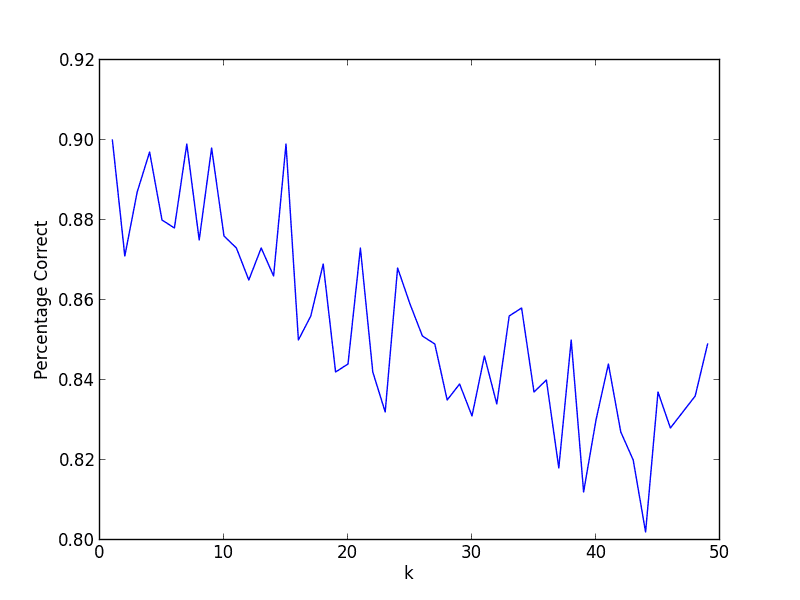
A run with $ k=1$ gives a surprisingly good 89% success rate. Varying $ k$, we see this is about as good as it gets without any modifications to the algorithm or the metric. Indeed, the graph below shows that the handwritten digits data set agrees with the axiom of neighborliness to a fair approximation.
Of course, there are many improvements we could make to this naive algorithm. But considering that it utilizes no domain knowledge and doesn’t manipulate the input data in any way, it’s not too shabby.
As a side note, it would be fun to get some tablet software and have it use this method to recognize numbers as one writes it. Alas, we have little time for these sorts of applications.
Advantages, Enhancements, and Problems
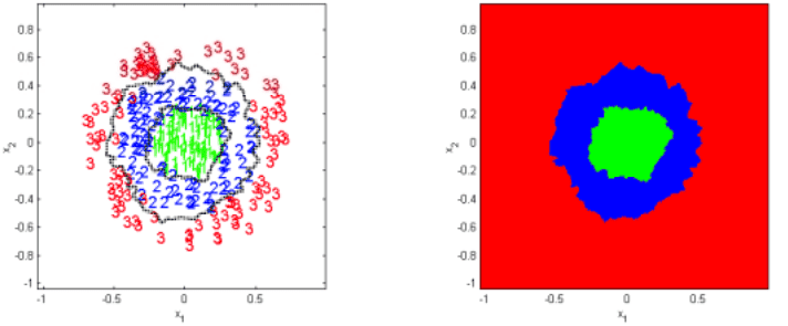
One reason k-nearest-neighbors is such a common and widely-known algorithm is its ease of implementation. Indeed, we implemented the core algorithm in a mere three lines of Python. On top of that, k-nearest-neighbors is pleasingly parallel, and inherently flexible. Unlike the Perceptron algorithm, which relies on linear separability, k-nearest-neighbors and the axiom of neighborliness allow for datasets with many different geometric structures. These lecture notes give a good example, as shown below, and the reader can surely conjure many more.
And of course, the flexibility is even greater by virtue of being able to use any metric for distance computations. One may, for instance, use the Manhattan metric if the points in question are locations in a city. Or if the data is sequential, one could use the dynamic time warping distance (which isn’t truly a metric, but is still useful). The possibilities are only limited by the discovery of new and useful metrics.
With such popularity, k-nearest-neighbors often comes with a number of modifications and enhancements. One enhancement is to heuristically remove certain points close to the decision boundary. This technique is called edited k-nearest-neighbors. Another is to weight certain features heavier in the distance computations, which requires one to programmatically determine which features help less with classification. This is getting close to the realm of a decision tree, and so we’ll leave this as an exercise to the reader.
The next improvement has to do with runtime. Given $ n$ training points and $ d$ features (d for dimension), one point requires $ O(nd)$ to classify. This is particularly expensive, because most of the distance computations performed are between points that are far away, and as $ k$ is usually small, they won’t influence in the classification.
One way to alleviate this is to store the data points in a data structure called a k-d tree. The k-d tree originated in computational geometry in the problem of point location. It partitions space into pieces based on the number of points in each resulting piece, and organizes the partitions into a tree. In other words, it will partition tightly where the points are dense, and loosely where the points are sparse. At each step of traversing the tree, one can check to see which sub-partition the unclassified point lies in, and descend appropriately. With certain guarantees, this reduces the computation to $ O(\log(n)d)$. Unfortunately, there are issues with large-dimensional spaces that are beyond the scope of this post. We plan to investigate k-d trees further in a future series on computational geometry.
The last issue we consider is in data scaling. Specifically, one needs to be very careful when converting the real world data into numerical data. We can think of each of the features as a random variable, and we want all of these random variables to have comparable variation. The reason is simply because we’re using spheres. One can describe k-nearest-neighbors as finding the smallest (filled-in) sphere centered at the unlabeled point containing $ k$ labeled data points, and using the most common of those labels to classify the new point. Of course, one can talk about “spheres” in any metric space; it’s just the set of all points within some fixed distance from the center (and this definition doesn’t depend on the dimension of the space). The important point is that a sphere has uniform length along every axis. If the data is scaled improperly, then the geometry of the sphere won’t mirror the geometry of the data, and the algorithm will flounder.
So now we’ve seen a smattering of topics about k-nearest-neighbors. We’d love to continue the discussion of modifications in the comments. Next time we’ll explore decision trees, and work with another data set. Until then!