Neurons, as an Extension of the Perceptron Model
In a previous post in this series we investigated the Perceptron model for determining whether some data was linearly separable. That is, given a data set where the points are labelled in one of two classes, we were interested in finding a hyperplane that separates the classes. In the case of points in the plane, this just reduced to finding lines which separated the points like this:
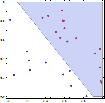
A hyperplane (the slanted line) separating the blue data points (class -1) from the red data points (class +1)
As we saw last time, the Perceptron model is particularly bad at learning data. More accurately, the Perceptron model is very good at learning linearly separable data, but most kinds of data just happen to more complicated. Even with those disappointing results, there are two interesting generalizations of the Perceptron model that have exploded into huge fields of research. The two generalizations can roughly be described as
- Use a number of Perceptron models in some sort of conjunction.
- Use the Perceptron model on some non-linear transformation of the data.
The point of both of these is to introduce some sort of non-linearity into the decision boundary. The first generalization leads to the neural network, and the second leads to the support vector machine. Obviously this post will focus entirely on the first idea, but we plan to cover support vector machines in the near future. Recall further that the separating hyperplane was itself defined by a single vector (a normal vector to the plane) $ \mathbf{w} = (w_1, \dots, w_n)$. To “decide” what class the new point $ \mathbf{x}$ is in, we check the sign of an inner product with an added constant shifting term:
\[ f(\mathbf{x}) = \textup{sign}(\left \langle \mathbf{w}, \mathbf{x} \right \rangle + b) = \textup{sign} \left ( b + \sum_{i=1}^n w_i x_i \right ) \]The class of a point is just the value of this function, and as we saw with the Perceptron this corresponds geometrically to which side of the hyperplane the point lies on. Now we can design a “neuron” based on this same formula. We consider a point $ \mathbf{x} = (x_1, \dots, x_n)$ to be an input to the neuron, and the output will be the sign of the above sum for some coefficients $ w_i$. In picture form it would look like this:
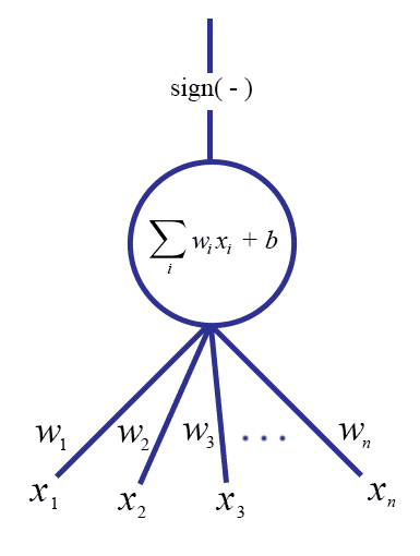
It is quite useful to literally think of this picture as a directed graph (see this blog’s gentle introduction to graph theory if you don’t know what a graph is). The edges corresponding to the coordinates of the input vector $ \mathbf{x}$ have weights $ w_i$, and the output edge corresponds to the sign of the linear combination. If we further enforce the inputs to be binary (that is, $ \mathbf{x} \in \left \{ 0, 1 \right \}^n$), then we get a very nice biological interpretation of the system. If we think of the unit as a neuron, then the input edges correspond to nerve impulses, which can either be on or off (identically to an electrical circuit: there is high current or low current). The weights $ w_i$ correspond to the strength of the neuronal connection. The neuron transmits or does not transmit a pulse as output depending on whether the inputs are strong enough.
We’re not quite done, though, because in this interpretation the output of the neuron will either fire or not fire. However, neurons in real life are somewhat more complicated. Specifically, neurons do not fire signals according to a discontinuous function. In addition, we want to use the usual tools from classical calculus to analyze our neuron, but we cannot do that unless the activation function is differentiable, and a prerequisite for that is to be continuous. In plain words, we need to allow our neurons to be able to “partially fire.” We need a small range at which the neuron ramps up quickly from not firing to firing, so that the activation function as a whole is differentiable.
This raises the obvious question: what function should we pick? It turns out that there are a number of possible functions we could use, ranging from polynomial to exponential in nature. But before we pick one in particular, let’s outline the qualities we want such a function to have.
Definition: A function $ \sigma: \mathbb{R} \to [0,1]$ is an activation function if it satisfies the following properties:
- It has a first derivative $ \sigma'$.
- $ \sigma$ is non-decreasing, that is $ \sigma'(x) \geq 0$ for all $ x$
- $ \sigma$ has horizontal asymptotes at both 0 and 1 (and as a consequence, $ \lim_{x \to \infty} \sigma(x) = 1$, and $ \lim_{x \to -\infty} \sigma(x) = 0$).
- $ \sigma$ and $ \sigma'$ are both computable functions.
With appropriate shifting and normalizing, there are a few reasonable (and time-tested) activation functions. The two main ones are the hyperbolic tangent $ \tanh(x)$ and the sigmoid curve $ 1/ (1+e^{-t})$. They both look (more or less) like this:

A sigmoid function (source: Wikipedia)
And it is easy to see visually that this is what we want.
As a side note, the sigmoid function is actually not used very often in practice for a good reason: it gets too “flat” when the function value approaches 0 or 1. The reason this is bad is because how “flat” the function is (the gradient) will guide the learning process. If the function is very flat, then the network won’t learn as quickly. This will manifest itself in our test later in this post, when we see that a neural network struggles to learn the sine function. It struggles specifically at those values of the function that are close to 1 or -1. Though I don’t want to go into too much detail about this, one alternative that has found a lot of success in deep learning is the “rectified linear unit.” This also breaks the assumption of having a derivative everywhere, so one needs a bit more work to deal with that.
Withholding any discussion of why one would pick one specific activation over another, there is one more small detail. In the Perceptron model we allowed a “bias” $ b$ which translated the separating hyperplane so that it need not pass through the origin, hence allowing a the set of all pairs $ (\mathbf{w}, b)$ to represent every possible hyperplane. Perhaps the simplest way to incorporate the bias into this model is to add another input $ x_0$ which is fixed to 1. Then we add a weight $ w_0$, and it is easy to see that the constant $ b$ can just be replaced with the weight $ w_0$. In other words, the inner product $ b \cdot 1 + \left \langle \mathbf{w}, \mathbf{x} \right \rangle$ is the same as the inner product of two new vectors $ \mathbf{w}', \mathbf{x}'$ where we set $ w'_0 = b$ and $ x'_0 = 1$ and $ w'_i = w_i, x'_i = x_i$ for all other $ i$.
The updated picture is now:
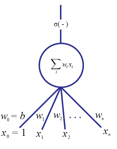
Now the specification of a single neuron is complete:
**Definition: **A neuron $ N$ is a pair $ (W, \sigma)$, where $ W$ is a list of weights $ (w_0, w_1, \dots, w_k)$, and $ \sigma$ is an activation function. The _impulse function o_f a neuron $ N$, which we will denote $ f_N: \left \{ 0,1 \right \}^{k+1} \to [0,1]$, is defined as
\[ f_N(\mathbf{x}) = \sigma(\left \langle \mathbf{w}, \mathbf{x} \right \rangle) = \sigma \left (\sum_{i=0}^k w_i x_i \right ) \]We call $ w_0$ the bias weight, and by convention the first input coordinate $ x_0$ is fixed to 1 for all inputs $ \mathbf{x}$.
(Since we always fix the first input to 1, $ f_N$ is technically a function $ \left \{ 0,1 \right \}^k \to \left \{ 0,1 \right \}$, but the reader will forgive us for blurring these details.)
Combining Neurons into a Network
The question of how to “train” a single neuron is just a reformulation of the Perceptron problem. If we have a data set $ \mathbf{x}_i$ with class labels $ y_i = \pm 1$, we want to update the weights of a neuron so that the outputs agree with their class labels; that is, $ f_N(\mathbf{x}_i) = y_i$ for all $ i$. And we saw in the Perceptron how to do this: it’s fast and efficient, given that the data are linearly separable. And in fact training a neuron in this model (accounting for the new activation function) will give us identical decision functions as in the Perceptron model. All we have done so far is change our perspective from geometry to biology. But as we mentioned originally, we want to form a mathematical army of neurons, all working together to form a more powerful decision function.
The question is what form should this army take? Since we already thought of a single neuron as a graph, let’s generalize this. Instead of having a bunch of “input” vertices, a single “output” vertex, and one neuron doing the computation, we now have the same set of input vertices, the same output vertex, but now a number of intermediate neurons connected arbitrarily to each other. That is, the edges that are outputs of some neurons are connected to the inputs of other neurons, and the very last neuron’s output is the final output. We call such a construction a neural network.
For example, the following graph gives a neural network with 5 neurons
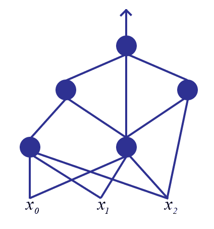
To compute the output of any neuron $ N$, we need to compute the values of the impulse functions for each neuron whose output feeds into $ N$. This in turn requires computing the values of the impulse functions for each of the inputs to those neurons, and so on. If we imagine electric current flowing through such a structure, we can view it as a kind of network flow problem, which is where the name “neural networks” comes from. This structure is also called a dependency graph, and (in the parlance of graph theory) a directed acyclic graph. Though nothing technical about these structures will show up in this particular post, we plan in the future to provide primers on their basic theories.
We remark that we view the above picture as a directed graph with the directed edges going upwards. And as in the picture, the incidence structure (which pairs of neurons are connected or not connected) of the graph is totally arbitrary, as long as it has no cycles. Note that this is in contrast to the classical idea of a neural network as “layered” with one or more intermediate layers, such that all neurons in neighboring layers are completely connected to one another. Hence we will take a slightly more general approach in this post.
Now the question of training a network of interconnected neurons is significantly more complicated than that of training a single neuron. The algorithm to do so is called backpropagation, because we will check to see if the final output is an error, and if it is we will propagate the error backward through the network, updating weights as we go. But before we get there, let’s explore some motivation for the algorithm.
The Backpropagation AlgorithmSingle Neuron
Let us return to the case of a single neuron $ N$ with weights $ \mathbf{w} = (w_0, \dots , w_k)$ and an input $ \mathbf{x} = (x_0, \dots, x_k)$. And momentarily, let us remove the activation function $ \sigma$ from the picture (so that $ f_N$ just computes the summation part). In this simplified world it is easy to take a given set of training inputs $ \mathbf{x}_j$ with labels $ y_j \in \left \{ 0,1 \right \}$ and compute the error of our neuron $ N$ on the entire training set. A standard mathematical way to compute error is by sum of the squared deviations of our neuron’s output from the actual label.
\[ E(\mathbf{w}) = \sum_j (y_jf_N(\mathbf{x}_j))^2 \]The important part is that $ E$ is a function just of the weights $ w_i$. In other words, the set of weights completely specifies the behavior of a single neuron.
Enter calculus. Any time we have a multivariate function (here, each of the weights $ w_i$ is a variable), then we can speak of its minima and maxima. In our case we strive to find a global minimum of the error function $ E$, for then we would have learned our target classification function as well as possible. Indeed, to improve upon our current set of weights, we can use the standard gradient-descent algorithm. We have discussed versions of the gradient-descent algorithm on this blog before, as in our posts on decrypting substitution ciphers with n-grams and finding optimal stackings in Texas Hold ‘Em. We didn’t work with calculus there because the spaces involved were all discrete. But here we will eventually extend this error function to allow the inputs $ x_i$ to be real-valued instead of binary, and so we need the full power of calculus. Luckily for the uninformed reader, the concept of gradient descent is the same in both cases. Since $ E$ gives us a real number for each possible neuron (each choice of weights), we can take our current neuron and make it better it by changing the weights slightly, and ensuring our change gives us a smaller value under $ E$. If we cannot ensure this, then we have reached a minimum.
Here are the details. For convenience we add a factor of $ 1/2$ to $ E$ and drop the subscript $ N$ from $ f_N$. Since minimizing $ E$ is the same as minimizing $ \frac{1}{2}E$, this changes nothing about the minima of the function. That is, we will henceforth work with
\[ E(\mathbf{w}) = \frac{1}{2} \sum_j (y_jf(\mathbf{x}_j))^2 \]Then we compute the gradient $ \nabla E$ of $ E$. For fixed values of the variables $ w_i$ (our current set of weights) this is a vector in $ \mathbb{R}^n$, and as we know from calculus it points in the direction of steepest ascent of the function $ E$. That is, if we subtract some sufficiently small multiple of this vector from our current weight vector, we will be closer to a minimum of the error function than we were before. If we were to add, we’d go toward a maximum.
Note that $ E$ is never negative, and so it will have a global minimum value at or near 0 (if it is possible for the neuron to represent the target function perfectly, it will be zero). That is, our update rule should be
\[ \mathbf{w}_\textup{current} = \mathbf{w}_\textup{current}\eta \nabla E(\mathbf{w}_\textup{current}) \]where $ \eta$ is some fixed parameter between 0 and 1 that represent the “learning rate.” We will not mention $ \eta$ too much except to say that as long as it is sufficiently small and we allow ourselves enough time to learn, we are guaranteed to get a good approximation of some local minimum (though it might not be a global one).
With this update rule it suffices to compute $ \nabla E$ explicitly.
\[ \nabla E = \left ( \frac{\partial E}{\partial w_0}, \dots, \frac{\partial E}{\partial w_n} \right ) \]In each partial $ \partial E / \partial w_i$ we consider each other variable beside $ w_i$ to be constant, and combining this with the chain rule gives
\[ \frac{\partial E}{\partial w_i} =\sum_j (y_jf(\mathbf{x}_j)) \frac{\partial f}{\partial w_i} \]Since in the summation formula for $ f$ the $ w_i$ variable only shows up in the product $ w_i x_{j,i}$ (where $ x_{j,i}$ is the $ i$-th term of the vector $ \mathbf{x}_j$), the last part expands as $ x_{j,i}$. i.e. we have
\[ \frac{\partial E}{\partial w_i} =\sum_j (y_jf(\mathbf{x}_j)) x_{j,i} \]Noting the negatives cancelling, this makes our update rule just
\[ w_i = w_i + \eta \sum_j (y_jf(\mathbf{x}_j))x_{j,i} \]There is an alternative form of an update rule that allows one to update the weights after each individual input is tested (as opposed to checking the outputs of the entire training set). This is called the stochastic update rule, and is given identically as above but without summing over all $ j$:
\[ \mathbf{w} = \mathbf{w} + \eta (y_jf(\mathbf{x}_j)) \mathbf{x}_j \]For our purposes in this post, the stochastic and non-stochastic update rules will give identical results.
Adding in the activation function $ \sigma$ is not hard, but we will choose our $ \sigma$ so that it has particularly nice computability properties. Specifically, we will pick $ \sigma = 1/(1+e^{-x})$ the sigmoid function, because it satisfies the identity
\[ \sigma'(x) = \sigma(x)(1-\sigma(x)) \]So instead of $ \partial f$ in the formula above we need $ \partial (\sigma \circ f) / \partial w_i$, and this requires the chain rule once again:
\[ \frac{\partial E}{\partial w_i} =\sum_j (y_j\sigma(f(\mathbf{x}_j))) \sigma'(f(\mathbf{x}_j))x_{j,i} \]And using the identity for $ \sigma'$ gives us
\[ \frac{\partial E}{\partial w_i} =\sum_j (y_j\sigma(f(\mathbf{x}_j))) \sigma(f(\mathbf{x}_j))(1-\sigma(f(\mathbf{x}_j)))x_{j,i} \]And a similar update rule as before. If we denote by $ o_j$ the output value $ \sigma(f(\mathbf{x}_j))$, then the stochastic version of this update rule is
\[ \mathbf{w} = \mathbf{w} + \eta o_j (1-o_j)(y_jo_j)\mathbf{x}_j \]Now that we have motivated an update rule for a single neuron, let’s see how to apply this to an entire network of neurons.
The Backpropagation AlgorithmEntire Network
There is a glaring problem in training a neural network using the update rule above. We don’t know what the “expected” output of any of the internal edges in the graph are. In order to compute the error we need to know what the correct output should be, but we don’t immediately have this information.
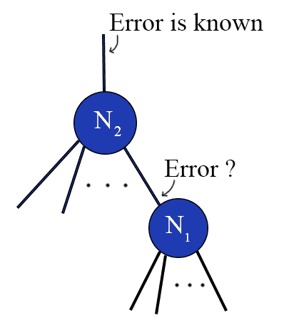
We don't know the error value for a non-output node in the network.
We don’t know the error value for a non-output node in the network.
In the picture above, we know the expected value of the edge leaving the node $ N_2$, but not that of $ N_1$. In order to compute the error for $ N_1$, we need to derive some kind of error value for nodes in the middle of the network.
It seems reasonable that the error for $ N_1$ should depend on the errors of the nodes for which $ N_1$ provides an input. That is, in the following picture the error should come from all of the neurons $ M_1, \dots M_n$.
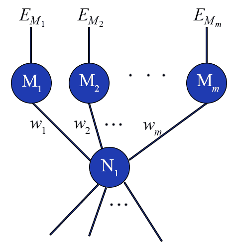
weightedsumerror
In particular, one possible error value for a particular input to the entire network $ \mathbf{x}$ would be a weighted sum over the errors of $ M_i$, where the weights are the weights of the edges from $ N_1$ to $ M_i$. In other words, if $ N_1$ has little effect on the output of one particular $ M_i$, it shouldn’t assume too much responsibility for that error. That is, using the above picture, the error for $ N_1$ (in terms of the input weights $ v_i$) is
\[ \sum_i w_i E_{M_i} \]where $ E_{M_i}$ is the error computed for the node $ M_i$.
It turns out that there is a nice theoretical justification for using this quantity as well. In particular, if we think of the entire network as a single function, we can imagine the error $ E(\mathbf{w})$ as being a very convoluted function of all the weights in the network. But no matter how confusing the function may be to write down, we know that it only involves addition, multiplication, and composition of differentiable functions. So if we want to know how to update the error with respect to a weight that is hidden very far down in the network, in theory it just requires enough applications of the chain rule to find it.
To see this, let’s say we have a nodes $ N_{1,k}$ connected forward to nodes $ N_{2,j}$ connected forward to nodes $ N_{3,i}$, such that the weights $ w_{k,j}$ represent weights going from $ N_{1,k} \to N_{2,j}$, and weights $ w_{j,i}$ are $ N_{2,j} \to N_{3,i}$.
If we want to know the partial derivative of $ E$ with respect to the deeply nested weight $ w_{k,j}$, then we can just compute it:
\[ \frac{\partial E}{\partial w_{k,j}} = -\sum_i (y_io_i)\frac{\partial o_i}{\partial w_{k,j}} \]where $ o_i = f_{N_{1,j}}(\dots) = \sigma(f(\dots))$ represents the value of the impulse function at each of the output neurons, in terms of a bunch of crazy summations we omit for clarity.
But after applying the chain rule, the partial of the inner summation $ f = \sum_j w_{j,i}x_k$ only depends on $ w_{k,j}$ via the coefficient $ w_{j,i}$. i.e., the weight $ w_{k,j}$ only affects node $ N_{3,i}$ by the output of $ N_{2,j}$ passing through the edge labeled $ w_{j,i}$. So we get a sum
\[ \frac{\partial E}{\partial w_{k,j}} = -\sum_i (y_io_i)\sigma'(f(\dots)) w_{j,i} \]That is, it’s simply a weighted sum of the final errors $ y_io_i$ by the right weights. The stuff inside the $ f(\dots)$ is simply the output of that node, which is again a sum over its inputs. In stochastic form, this makes our update rule (for the weights of $ N_j$) just
\[ \mathbf{w} = \mathbf{w} + \eta o_j(1-o_j) \left ( \sum_i w_{j,i} (y_io_i) \right ) \mathbf{z} \]where by $ \mathbf{z}$ we denote the vector of inputs to the neuron in question (these may be the original input $ \mathbf{x}$ if this neuron is the first in the network and all of the inputs are connected to it, or it may be the outputs of other neurons feeding into it).
The argument we gave only really holds for a network where there are only two edges from the input to the output. But the reader who has mastered the art of juggling notation may easily generalize this via induction to prove it in general. This really is a sensible weight update for any neuron in the network.
And now that we have established our update rule, the backpropagation algorithm for training a neural network becomes relatively straightforward. Start by initializing the weights in the network at random. Evaluate an input $ \mathbf{x}$ by feeding it forward through the network and recording at each internal node the output value $ o_j$, and call the final output $ o$. Then compute the error for that output value, propagate the error back to each of the nodes feeding into the output node, and update the weights for the output node using our update rule. Repeat this error propagation followed by a weight update for each of the nodes feeding into the output node in the same way, compute the updates for the nodes feeding into those nodes, and so on until the weights of the entire network are updated. Then repeat with a new input $ \mathbf{x}$.
One minor issue is when to stop. Specifically, it won’t be the case that we only need to evaluate each input $ \mathbf{x}$ exactly once. Depending on how the learning parameter $ \eta$ is set, we may need to evaluate the entire training set many times! Indeed, we should only stop when the gradient for all of our examples is small, or we have run it for long enough to exhaust our patience. For simplicity we will ignore checking for a small gradient, and we will simply fix a number of iterations. We leave the gradient check as an exercise to the reader.
Then the result is a trained network, which we can further use to evaluate the labels for unknown inputs.
Python Implementation
We now turn to implementing a neural network. As usual, all of the source code used in this post (and then some) is available on this blog’s Github page.
The first thing we need to implement all of this is a data structure for a network. That is, we need to represent nodes and edges connecting nodes. Moreover each edge needs to have an associated value, and each node needs to store multiple values (the error that has been propagated back, and the output produced at that node). So we will represent this via two classes:
class Node:
   def __init__(self):
      self.lastOutput = None
      self.lastInput = None
      self.error = None
      self.outgoingEdges = []
      self.incomingEdges = []

class Edge:
   def __init__(self, source, target):
      self.weight = random.uniform(0,1)
      self.source = source
      self.target = target

      # attach the edges to its nodes
      source.outgoingEdges.append(self)
      target.incomingEdges.append(self)
Then a neural network is represented by the set of input and output nodes.
class Network:
   def __init__(self):
      self.inputNodes = []
      self.outputNode = None
In particular, each Node needs to know about its most recent output, input, and error in order to update its weights. So any time we evaluate some input, we need to store these values in the Node. We will progressively fill in these classes with the methods needed to evaluate and train the network on data. But before we can do anything, we need to be able to distinguish between an input node and a node internal to the network. For this we create a subclass of Node called InputNode:
class InputNode(Node):
   def __init__(self, index):
      Node.__init__(self)
      self.index = index; # the index of the input vector corresponding to this node
And now here is a function which evaluates a given input when provided a neural network:
class Network:
   ...

   def evaluate(self, inputVector):
      return self.outputNode.evaluate(inputVector)

class Node:
   ...

   def evaluate(self, inputVector):
      self.lastInput = []
      weightedSum = 0

      for e in self.incomingEdges:
         theInput = e.source.evaluate(inputVector)
         self.lastInput.append(theInput)
         weightedSum += e.weight * theInput

      self.lastOutput = activationFunction(weightedSum)
      return self.lastOutput

class InputNode(Node):
   ...

   def evaluate(self, inputVector):
      self.lastOutput = inputVector[self.index]
      return self.lastOutput
A network calls the evaluate function on its output node, and each node recursively calls evaluate on the sources of each of its incoming edges. An InputNode simply returns the corresponding entry in the inputVector (which requires us to pass the input vector along through the recursive calls). Since our graph structure is arbitrary, we note that some nodes may be “evaluated” more than once per evaluation. As such, we need to store the node’s output for the duration of the evaluation. We also need to store this value for use in training, and so before a call to evaluate we must clear this value. We omit the details here for brevity.
We will use the evaluate() function for training as well as for evaluating unknown inputs. As usual, examples of using these classes (and tests) are available in the full source code on this blog’s Github page.
In addition, we need to automatically add bias nodes and corresponding edges to the non-input nodes. This results in a new subclass of Node which has a default evaluate() value of 1. Because of the way we organized things, the existence of this class changes nothing about the training algorithm.
class BiasNode(InputNode):
   def __init__(self):
      Node.__init__(self)

   def evaluate(self, inputVector):
      return 1.0
We simply add a function to the Node class (which is overridden in the InputNode class) which adds a bias node and edge to every non-input node. The details are trivial; the reader may see them in the full source code.
The training algorithm will come in a loop consisting of three steps: first, evaluate an input example. Second, go through the network updating the error values of each node using backpropagation. Third, go through the network again to update the weights of the edges appropriately. This can be written as a very short function on a Network, which then requires a number of longer functions on the Node classes:
class Network:
   ...

   def propagateError(self, label):
      for node in self.inputNodes:
         node.getError(label)

   def updateWeights(self, learningRate):
      for node in self.inputNodes:
         node.updateWeights(learningRate)

   def train(self, labeledExamples, learningRate=0.9, maxIterations=10000):
      while maxIterations > 0:
         for example, label in labeledExamples:
            output = self.evaluate(example)
            self.propagateError(label)
            self.updateWeights(learningRate)

            maxIterations -= 1
That is, the network class just makes the first call for each of these recursive processes. We then have the following functions on Nodes to implement getError and updateWeights:
class InputNode(Node):
   ...

   def updateWeights(self, learningRate):
      for edge in self.outgoingEdges:
         edge.target.updateWeights(learningRate)

   def getError(self, label):
      for edge in self.outgoingEdges:
         edge.target.getError(label)

class Node:
   ...

   def getError(self, label):
      if self.error is not None:
         return self.error

      if self.outgoingEdges == []: # this is an output node
         self.error = label - self.lastOutput
      else:
         self.error = sum([edge.weight * edge.target.getError(label)
                           for edge in self.outgoingEdges])

      return self.error

   def updateWeights(self, learningRate):
      if (self.error is not None and self.lastOutput is not None
            and self.lastInput is not None):

         for i, edge in enumerate(self.incomingEdges):
            edge.weight += (learningRate * self.lastOutput * (1 - self.lastOutput) *
                           self.error * self.lastInput[i])

         for edge in self.outgoingEdges:
            edge.target.updateWeights(learningRate)

         self.error = None
         self.lastInput = None
         self.lastOutput = None
These are simply the formulas we derived in the previous sections translated into code. The propagated error is computed as a weighted sum in getError(), and the previous input and output values were saved from the call to evaluate().
A Sine Curve Example, and Issues
One simple example we can use to illustrate this is actually not a decision problem, per se, but a function estimation problem. In the course of all of this calculus, we implicitly allowed our neural network to output any values between 0 and 1 (indeed, the activation function did this for us). And so we can use a neural network to approximate any function which has values in $ [0,1]$. In particular we will try this on
\[ \displaystyle f(x) = \frac{1}{2}(\sin(x) + 1) \]on the domain $ [0,4 \pi ]$.
Our network is simple: we have a single layer of twenty neurons, each of which is connected to a single input neuron and a single output neuron. The learning rate is set to 0.25, the number of iterations is set to a hundred thousand, and the training set is randomly sampled from the domain.
After training (which takes around fifteen seconds), the average error (when tested against a new random sample) is between 0.03 and 0.06. Here is an example of one such output:
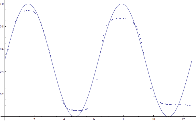
An example of a 20-node neural network approximating two periods of a sine function.
An example of a 20-node neural network approximating two periods of a sine function.
This picture hints at an important shortcoming of our algorithm. Note how the neural network’s approximation of the sine function does particularly poorly close to 0 and 1. This is not a coincidence, but rather a side effect of our activation function $ \sigma$. In particular, because the sigmoid function achieves the values 0 and 1 only in the limit. That is, they never actually achieve 0 and 1, and in order to get close we require prohibitively large weights (which in turn correspond to rather large values to be fed to the activation function). One potential solution is to modify our sine function slightly more, by scaling it and translating it so that its values lie in $ [0.1, 0.9]$, say. We leave this as an exercise to the reader.
As one might expect, the neural network also does better when we test it on a single period instead of two (since the sine function is less “complicated” on a single period). We also constructed a data set of binary numbers whose labels were 1 if the number was even and 0 if the number was odd. A similar layout to the sine example with three internal nodes again gave good results.
The issues arise on larger datasets. One big problem with training a neural network is that it’s near impossible to determine the “correct” structure of the network ahead of time. The success of our sine function example, for instance, depended much more than we anticipated on the number of nodes used. Of course, this also depends on the choice of learning rate and the number of iterations allowed, but the point is the same: the neural network is fraught with arbitrary choices. What’s worse is that it’s just as impossible to tell if your choices are justified. All you have is an empirical number to determine how well your network does on one training set, and inspecting the values of the various weights will tell you nothing in all but the most trivial of examples.
There are a number of researchers who have attempted to alleviate this problem in some way. One prominent example is the Cascade Correlation algorithm, which dynamically builds the network structure depending on the data. Other avenues include dynamically updating the learning rate and using a variety of other activation and error functions, based on information theory and game theory (adding penalties for various undesirable properties). Still other methods involve alternative weight updates based on more advanced optimization techniques (such as the conjugate gradient method). Part of the benefit of the backpropagation algorithm is that the choice of error function is irrelevant, as long as it is differentiable. This gives us a lot of flexibility to customize the neural network for our own application domain.
These sorts of questions are what have caused neural networks to become such a huge field of research in machine learning. As such, this blog post has only given the reader a small taste of what is out there. This is the bread and butter in a world of fine cuisine: it’s proven to be a solid choice, but it leaves a cornucopia of flavors unrealized and untapped.
The future of this machine learning series, however, will deviate from the neural network path. We will instead investigate the other extension of the Perceptron model, the Support Vector Machine. We will also lay down some formal theories of learning, because as of yet we have simply been exploring algorithms without the ability to give guarantees on their performance. In order to do that, we must needs formalize the notion of an algorithm “learning” a task. This is no small feat, and nobody has quite agreed on the best formalization. We will nevertheless explore these frameworks, and see what kinds of theorems we can prove in them.
Until then!
Want to respond? Send me an email, post a webmention, or find me elsewhere on the internet.