It is a wonder that we have yet to officially write about probability theory on this blog. Probability theory underlies a huge portion of artificial intelligence, machine learning, and statistics, and a number of our future posts will rely on the ideas and terminology we lay out in this post. Our first formal theory of machine learning will be deeply ingrained in probability theory, we will derive and analyze probabilistic learning algorithms, and our entire treatment of mathematical finance will be framed in terms of random variables.
And so it’s about time we got to the bottom of probability theory. In this post, we will begin with a naive version of probability theory. That is, everything will be finite and framed in terms of naive set theory without the aid of measure theory. This has the benefit of making the analysis and definitions simple. The downside is that we are restricted in what kinds of probability we are allowed to speak of. For instance, we aren’t allowed to work with probabilities defined on all real numbers. But for the majority of our purposes on this blog, this treatment will be enough. Indeed, most programming applications restrict infinite problems to finite subproblems or approximations (although in their analysis we often appeal to the infinite).
We should make a quick disclaimer before we get into the thick of things: this primer is not meant to connect probability theory to the real world. Indeed, to do so would be decidedly unmathematical. We are primarily concerned with the mathematical formalisms involved in the theory of probability, and we will leave the philosophical concerns and applications to future posts. The point of this primer is simply to lay down the terminology and basic results needed to discuss such topics to begin with.
So let us begin with probability spaces and random variables.
Finite Probability Spaces
We begin by defining probability as a set with an associated function. The intuitive idea is that the set consists of the outcomes of some experiment, and the function gives the probability of each event happening. For example, a set $ \left \{ 0,1 \right \}$ might represent heads and tails outcomes of a coin flip, while the function assigns a probability of one half (or some other numbers) to the outcomes. As usual, this is just intuition and not rigorous mathematics. And so the following definition will lay out the necessary condition for this probability to make sense.
Definition: A finite set $ \Omega$ equipped with a function $ f: \Omega \to [0,1]$ is a probability space if the function $ f$ satisfies the property
$$\displaystyle \sum_{\omega \in \Omega} f(\omega) = 1$$That is, the sum of all the values of $ f$ must be 1.
Sometimes the set $ \Omega$ is called the sample space, and the act of choosing an element of $ \Omega$ according to the probabilities given by $ f$ is called drawing an example. The function $ f$ is usually called the probability mass function. Despite being part of our first definition, the probability mass function is relatively useless except to build what follows. Because we don’t really care about the probability of a single outcome as much as we do the probability of an event.
Definition: An event $ E \subset \Omega$ is a subset of a sample space.
For instance, suppose our probability space is $ \Omega = \left \{ 1, 2, 3, 4, 5, 6 \right \}$ and $ f$ is defined by setting $ f(x) = 1/6$ for all $ x \in \Omega$ (here the “experiment” is rolling a single die). Then we are likely interested in more exquisite kinds of outcomes; instead of asking the probability that the outcome is 4, we might ask what is the probability that the outcome is even? This event would be the subset $ \left \{ 2, 4, 6 \right \}$, and if any of these are the outcome of the experiment, the event is said to occur. In this case we would expect the probability of the die roll being even to be 1/2 (but we have not yet formalized why this is the case).
As a quick exercise, the reader should formulate a two-dice experiment in terms of sets. What would the probability space consist of as a set? What would the probability mass function look like? What are some interesting events one might consider (if playing a game of craps)?
Of course, we want to extend the probability mass function $ f$ (which is only defined on single outcomes) to all possible events of our probability space. That is, we want to define a probability measure $ \textup{P}: 2^\Omega \to \mathbb{R}$, where $ 2^\Omega$ denotes the set of all subsets of $ \Omega$. The example of a die roll guides our intuition: the probability of any event should be the sum of the probabilities of the outcomes contained in it. i.e. we define
$$\displaystyle \textup{P}(E) = \sum_{e \in E} f(e)$$where by convention the empty sum has value zero. Note that the function $ \textup{P}$ is often denoted $ \textup{Pr}$.
So for example, the coin flip experiment can’t have zero probability for both of the two outcomes 0 and 1; the sum of the probabilities of all outcomes must sum to 1. More coherently: $ \textup{P}(\Omega) = \sum_{\omega \in \Omega} f(\omega) = 1$ by the defining property of a probability space. And so if there are only two outcomes of the experiment, then they must have probabilities $ p$ and $ 1-p$ for some $ p$. Such a probability space is often called a Bernoulli trial.
Now that the function $ \textup{P}$ is defined on all events, we can simplify our notation considerably. Because the probability mass function $ f$ uniquely determines $ \textup{P}$ and because $ \textup{P}$ contains all information about $ f$ in it ($ \textup{P}(\left \{ \omega \right \}) = f(\omega)$), we may speak of $ \textup{P}$ as the probability measure of $ \Omega$, and leave $ f$ out of the picture. Of course, when we define a probability measure, we will allow ourselves to just define the probability mass function and the definition of $ \textup{P}$ is understood as above.
There are some other quick properties we can state or prove about probability measures: $ \textup{P}(\left \{ \right \}) = 0$ by convention, if $ E, F$ are disjoint then $ \textup{P}(E \cup F) = \textup{P}(E) + \textup{P}(F)$, and if $ E \subset F \subset \Omega$ then $ \textup{P}(E) \leq \textup{P}(F)$. The proofs of these facts are trivial, but a good exercise for the uncomfortable reader to work out.
Random Variables
The next definition is crucial to the entire theory. In general, we want to investigate many different kinds of random quantities on the same probability space. For instance, suppose we have the experiment of rolling two dice. The probability space would be
$$\displaystyle \Omega = \left \{ (1,1), (1,2), (1,3), \dots, (6,4), (6,5), (6,6) \right \}$$Where the probability measure is defined uniformly by setting all single outcomes to have probability 1/36. Now this probability space is very general, but rarely are we interested only in its events. If this probability space were interpreted as part of a game of craps, we would likely be more interested in the sum of the two dice than the actual numbers on the dice. In fact, we are really more interested in the payoff determined by our roll.
Sums of numbers on dice are certainly predictable, but a payoff can conceivably be any function of the outcomes. In particular, it should be a function of $ \Omega$ because all of the randomness inherent in the game comes from the generation of an output in $ \Omega$ (otherwise we would define a different probability space to begin with).
And of course, we can compare these two different quantities (the amount of money and the sum of the two dice) within the framework of the same probability space. This “quantity” we speak of goes by the name of a random variable.
Definition: A random variable $ X$ is a real-valued function on the sample space $ \Omega \to \mathbb{R}$.
So for example the random variable for the sum of the two dice would be $ X(a,b) = a+b$. We will slowly phase out the function notation as we go, reverting to it when we need to avoid ambiguity.
We can further define the set of all random variables $ \textup{RV}(\Omega)$. It is important to note that this forms a vector space. For those readers unfamiliar with linear algebra, the salient fact is that we can add two random variables together and multiply them by arbitrary constants, and the result is another random variable. That is, if $ X, Y$ are two random variables, so is $ aX + bY$ for real numbers $ a, b$. This function operates linearly, in the sense that its value is $ (aX + bY)(\omega) = aX(\omega) + bY(\omega)$. We will use this property quite heavily, because in most applications the analysis of a random variable begins by decomposing it into a combination of simpler random variables.
Of course, there are plenty of other things one can do to functions. For example, $ XY$ is the product of two random variables (defined by $ XY(\omega) = X(\omega)Y(\omega)$) and one can imagine such awkward constructions as $ X/Y$ or $ X^Y$. We will see in a bit why it these last two aren’t often used (it is difficult to say anything about them).
The simplest possible kind of random variable is one which identifies events as either occurring or not. That is, for an event $ E$, we can define a random variable which is 0 or 1 depending on whether the input is a member of $ E$. That is,
Definition: An indicator random variable $ 1_E$ is defined by setting $ 1_E(\omega) = 1$ when $ \omega \in E$ and 0 otherwise. A common abuse of notation for singleton sets is to denote $ 1_{\left \{ \omega \right \} }$ by $ 1_\omega$.
This is what we intuitively do when we compute probabilities: to get a ten when rolling two dice, one can either get a six, a five, or a four on the first die, and then the second die must match it to add to ten.
The most important thing about breaking up random variables into simpler random variables will make itself clear when we see that expected value is a linear functional. That is, probabilistic computations of linear combinations of random variables can be computed by finding the values of the simpler pieces. We can’t yet make that rigorous though, because we don’t yet know what it means to speak of the probability of a random variable’s outcome.
Definition: Denote by $ \left \{ X = k \right \}$ the set of outcomes $ \omega \in \Omega$ for which $ X(\omega) = k$. With the function notation, $ \left \{ X = k \right \} = X^{-1}(k)$.
This definition extends to constructing ranges of outcomes of a random variable. i.e., we can define $ \left \{ X < 5 \right \}$ or $ \left \{ X \textup{ is even} \right \}$ just as we would naively construct sets. It works in general for any subset of $ S \subset \mathbb{R}$. The notation is $ \left \{ X \in S \right \} = X^{-1}(S)$, and we will also call these sets events. The notation becomes useful and elegant when we combine it with the probability measure $ \textup{P}$. That is, we want to write things like $ \textup{P}(X \textup{ is even})$ and read it in our head “the probability that $ X$ is even”.
This is made rigorous by simply setting
$$\displaystyle \textup{P}(X \in S) = \sum_{\omega \in X^{-1}(S)} \textup{P}(\omega)$$In words, it is just the sum of the probabilities that individual outcomes will have a value under $ X$ that lands in $ S$. We will also use for $ \textup{P}(\left \{ X \in S \right \} \cap \left \{ Y \in T \right \})$ the shorthand notation $ \textup{P}(X \in S, Y \in T)$ or $ \textup{P}(X \in S \textup{ and } Y \in T)$.
Often times $ \left \{ X \in S \right \}$ will be smaller than $ \Omega$ itself, even if $ S$ is large. For instance, let the probability space be the set of possible lottery numbers for one week’s draw of the lottery (with uniform probabilities), let $ X$ be the profit function. Then $ \textup{P}(X > 0)$ is very small indeed.
We should also note that because our probability spaces are finite, the image of the random variable $ \textup{im}(X)$ is a finite subset of real numbers. In other words, the set of all events of the form $ \left \{ X = x_i \right \}$ where $ x_i \in \textup{im}(X)$ form a partition of $ \Omega$. As such, we get the following immediate identity:
$$\displaystyle 1 = \sum_{x_i \in \textup{im} (X)} P(X = x_i)$$The set of such events is called the probability distribution of the random variable $ X$.
The final definition we will give in this section is that of independence. There are two separate but nearly identical notions of independence here. The first is that of two events. We say that two events $ E,F \subset \Omega$ are independent if the probability of both $ E, F$ occurring is the product of the probabilities of each event occurring. That is, $ \textup{P}(E \cap F) = \textup{P}(E)\textup{P}(F)$. There are multiple ways to realize this formally, but without the aid of conditional probability (more on that next time) this is the easiest way. One should note that this is distinct from $ E,F$ being disjoint as sets, because there may be a zero-probability outcome in both sets.
The second notion of independence is that of random variables. The definition is the same idea, but implemented using events of random variables instead of regular events. In particular, $ X,Y$ are independent random variables if
$$\displaystyle \textup{P}(X = x, Y = y) = \textup{P}(X=x)\textup{P}(Y=y)$$for all $ x,y \in \mathbb{R}$.
Expectation
We now turn to notions of expected value and variation, which form the cornerstone of the applications of probability theory.
Definition: Let $ X$ be a random variable on a finite probability space $ \Omega$. The expected value of $ X$, denoted $ \textup{E}(X)$, is the quantity
$$\displaystyle \textup{E}(X) = \sum_{\omega \in \Omega} X(\omega) \textup{P}(\omega)$$Note that if we label the image of $ X$ by $ x_1, \dots, x_n$ then this is equivalent to
$$\displaystyle \textup{E}(X) = \sum_{i=1}^n x_i \textup{P}(X = x_i)$$The most important fact about expectation is that it is a linear functional on random variables. That is,
Theorem: If $ X,Y$ are random variables on a finite probability space and $ a,b \in \mathbb{R}$, then
$$\displaystyle \textup{E}(aX + bY) = a\textup{E}(X) + b\textup{E}(Y)$$Proof. The only real step in the proof is to note that for each possible pair of values $ x, y$ in the images of $ X,Y$ resp., the events $ E_{x,y} = \left \{ X = x, Y=y \right \}$ form a partition of the sample space $ \Omega$. That is, because $ aX + bY$ has a constant value on $ E_{x,y}$, the second definition of expected value gives
$$\displaystyle \textup{E}(aX + bY) = \sum_{x \in \textup{im} (X)} \sum_{y \in \textup{im} (Y)} (ax + by) \textup{P}(X = x, Y = y)$$and a little bit of algebraic elbow grease reduces this expression to $ a\textup{E}(X) + b\textup{E}(Y)$. We leave this as an exercise to the reader, with the additional note that the sum $ \sum_{y \in \textup{im}(Y)} \textup{P}(X = x, Y = y)$ is identical to $ \textup{P}(X = x)$. $ \square$
If we additionally know that $ X,Y$ are independent random variables, then the same technique used above allows one to say something about the expectation of the product $ \textup{E}(XY)$ (again by definition, $ XY(\omega) = X(\omega)Y(\omega)$). In this case $ \textup{E}(XY) = \textup{E}(X)\textup{E}(Y)$. We leave the proof as an exercise to the reader.
Now intuitively the expected value of a random variable is the “center” of the values assumed by the random variable. It is important, however, to note that the expected value need not be a value assumed by the random variable itself; that is, it might not be true that $ \textup{E}(X) \in \textup{im}(X)$. For instance, in an experiment where we pick a number uniformly at random between 1 and 4 (the random variable is the identity function), the expected value would be:
$$\displaystyle 1 \cdot \frac{1}{4} + 2 \cdot \frac{1}{4} + 3 \cdot \frac{1}{4} + 4 \cdot \frac{1}{4} = \frac{5}{2}$$But the random variable never achieves this value. Nevertheless, it would not make intuitive sense to call either 2 or 3 the “center” of the random variable (for both 2 and 3, there are two outcomes on one side and one on the other).
Let’s see a nice application of the linearity of expectation to a purely mathematical problem. The power of this example lies in the method: after a shrewd decomposition of a random variable $ X$ into simpler (usually indicator) random variables, the computation of $ \textup{E}(X)$ becomes trivial.
A tournament $ T$ is a directed graph in which every pair of distinct vertices has exactly one edge between them (going one direction or the other). We can ask whether such a graph has a Hamiltonian path, that is, a path through the graph which visits each vertex exactly once. The datum of such a path is a list of numbers $ (v_1, \dots, v_n)$, where we visit vertex $ v_i$ at stage $ i$ of the traversal. The condition for this to be a valid Hamiltonian path is that $ (v_i, v_{i+1})$ is an edge in $ T$ for all $ i$.
Now if we construct a tournament on $ n$ vertices by choosing the direction of each edges independently with equal probability 1/2, then we have a very nice probability space and we can ask what is the expected number of Hamiltonian paths. That is, $ X$ is the random variable giving the number of Hamiltonian paths in such a randomly generated tournament, and we are interested in $ \textup{E}(X)$.
To compute this, simply note that we can break $ X = \sum_p X_p$, where $ p$ ranges over all possible lists of the vertices. Then $ \textup{E}(X) = \sum_p \textup{E}(X_p)$, and it suffices to compute the number of possible paths and the expected value of any given path. It isn’t hard to see the number of paths is $ n!$ as this is the number of possible lists of $ n$ items. Because each edge direction is chosen with probability 1/2 and they are all chosen independently of one another, the probability that any given path forms a Hamiltonian path depends on whether each edge was chosen with the correct orientation. That’s just
$$\textup{P}(\textup{first edge and second edge and } \dots \textup{ and last edge})$$which by independence is
$$\displaystyle \prod_{i = 1}^n \textup{P}(i^\textup{th} \textup{ edge is chosen}) = \frac{1}{2^{n-1}}$$That is, the expected number of Hamiltonian paths is $ n!2^{-(n-1)}$.
Variance and Covariance
Just as expectation is a measure of center, variance is a measure of spread. That is, variance measures how thinly distributed the values of a random variable $ X$ are throughout the real line.
Definition: The variance of a random variable $ X$ is the quantity $ \textup{E}((X – \textup{E}(X))^2)$.
That is, $ \textup{E}(X)$ is a number, and so $ X – \textup{E}(X)$ is the random variable defined by $ (X – \textup{E}(X))(\omega) = X(\omega) – \textup{E}(X)$. It is the expectation of the square of the deviation of $ X$ from its expected value.
One often denotes the variance by $ \textup{Var}(X)$ or $ \sigma^2$. The square is for silly reasons: the standard deviation, denoted $ \sigma$ and equivalent to $ \sqrt{\textup{Var}(X)}$ has the same “units” as the outcomes of the experiment and so it’s preferred as the “base” frame of reference by some. We won’t bother with such physical nonsense here, but we will have to deal with the notation.
The variance operator has a few properties that make it quite different from expectation, but nonetheless fall our directly from the definition. We encourage the reader to prove a few:
- $ \textup{Var}(X) = \textup{E}(X^2) – \textup{E}(X)^2$.
- $ \textup{Var}(aX) = a^2\textup{Var}(X)$.
- When $ X,Y$ are independent then variance is additive: $ \textup{Var}(X+Y) = \textup{Var}(X) + \textup{Var}(Y)$.
- Variance is invariant under constant additives: $ \textup{Var}(X+c) = \textup{Var}(X)$.
In addition, the quantity $ \textup{Var}(aX + bY)$ is more complicated than one might first expect. In fact, to fully understand this quantity one must create a notion of correlation between two random variables. The formal name for this is covariance.
Definition: Let $ X,Y$ be random variables. The covariance of $ X$ and $ Y$, denoted $ \textup{Cov}(X,Y)$, is the quantity $ \textup{E}((X – \textup{E}(X))(Y – \textup{E}(Y)))$.
Note the similarities between the variance definition and this one: if $ X=Y$ then the two quantities coincide. That is, $ \textup{Cov}(X,X) = \textup{Var}(X)$.
There is a nice interpretation to covariance that should accompany every treatment of probability: it measures the extent to which one random variable “follows” another. To make this rigorous, we need to derive a special property of the covariance.
Theorem: Let $ X,Y$ be random variables with variances $ \sigma_X^2, \sigma_Y^2$. Then their covariance is at most the product of the standard deviations in magnitude:
$$|\textup{Cov}(X,Y)| \leq \sigma_X \sigma_Y$$Proof. Take any two non-constant random variables $ X$ and $ Y$ (we will replace these later with $ X – \textup{E}(X), Y – \textup{E}(Y)$). Construct a new random variable $ (tX + Y)^2$ where $ t$ is a real variable and inspect its expected value. Because the function is squared, its values are all nonnegative, and hence its expected value is nonnegative. That is, $ \textup{E}((tX + Y)^2)$. Expanding this and using linearity gives
$$\displaystyle f(t) = t^2 \textup{E}(X^2) + 2t \textup{E}(XY) + \textup{E}(Y^2) \geq 0$$This is a quadratic function of a single variable $ t$ which is nonnegative. From elementary algebra this means the discriminant is at most zero. i.e.
$$\displaystyle 4 \textup{E}(XY)^2 – 4 \textup{E}(X^2) \textup{E}(Y^2) \leq 0$$and so dividing by 4 and replacing $ X,Y$ with $ X – \textup{E}(X), Y – \textup{E}(Y)$, resp., gives
$$\textup{Cov}(X,Y)^2 \leq \sigma_X^2 \sigma_Y^2$$and the result follows. $ \square$
Note that equality holds in the discriminant formula precisely when $ Y = -tX$ (the discriminant is zero), and after the replacement this translates to $ Y – \textup{E}(Y) = -t(X – \textup{E}(X))$ for some fixed value of $ t$. In other words, for some real numbers $ a,b$ we have $ Y = aX + b$.
This has important consequences even in English: the covariance is maximized when $ Y$ is a linear function of $ X$, and otherwise is bounded from above and below. By dividing both sides of the inequality by $ \sigma_X \sigma_Y$ we get the following definition:
Definition: The Pearson correlation coefficient of two random variables $ X,Y$ is defined by
$$\displaystyle r= \frac{\textup{Cov}(X,Y)}{\sigma_X \sigma_Y}$$If $ r$ is close to 1, we call $ X$ and $ Y$ positively correlated. If $ r$ is close to -1 we call them negatively correlated, and if $ r$ is close to zero we call them uncorrelated.
The idea is that if two random variables are positively correlated, then a higher value for one variable (with respect to its expected value) corresponds to a higher value for the other. Likewise, negatively correlated variables have an inverse correspondence: a higher value for one correlates to a lower value for the other. The picture is as follows:
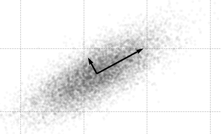
covariance
The horizontal axis plots a sample of values of the random variable $ X$ and the vertical plots a sample of $ Y$. The linear correspondence is clear. Of course, all of this must be taken with a grain of salt: this correlation coefficient is only appropriate for analyzing random variables which have a linear correlation. There are plenty of interesting examples of random variables with non-linear correlation, and the Pearson correlation coefficient fails miserably at detecting them.
Here are some more examples of Pearson correlation coefficients applied to samples drawn from the sample spaces of various (continuous, but the issue still applies to the finite case) probability distributions:

Various examples of the Pearson correlation coefficient, credit Wikipedia.
Though we will not discuss it here, there is still a nice precedent for using the Pearson correlation coefficient. In one sense, the closer that the correlation coefficient is to 1, the better a linear predictor will perform in “guessing” values of $ Y$ given values of $ X$ (same goes for -1, but the predictor has negative slope).
But this strays a bit far from our original point: we still want to find a formula for $ \textup{Var}(aX + bY)$. Expanding the definition, it is not hard to see that this amounts to the following proposition:
Proposition: The variance operator satisfies
$$\displaystyle \textup{Var}(aX+bY) = a^2\textup{Var}(X) + b^2\textup{Var}(Y) + 2ab \textup{Cov}(X,Y)$$And using induction we get a general formula:
$$\displaystyle \textup{Var} \left ( \sum_{i=1}^n a_i X_i \right ) = \sum_{i=1}^n \sum_{j = 1}^n a_i a_j \textup{Cov}(X_i,X_j)$$Note that in the general sum, we get a bunch of terms $ \textup{Cov}(X_i,X_i) = \textup{Var}(X_i)$.
Another way to look at the linear relationships between a collection of random variables is via a covariance matrix.
Definition: The covariance matrix of a collection of random variables $ X_1, \dots, X_n$ is the matrix whose $ (i,j)$ entry is $ \textup{Cov}(X_i,X_j)$.
As we have already seen on this blog in our post on eigenfaces, one can manipulate this matrix in interesting ways. In particular (and we may be busting out an unhealthy dose of new terminology here), the covariance matrix is symmetric and nonnegative, and so by the spectral theorem it has an orthonormal basis of eigenvectors, which allows us to diagonalize it. In more direct words: we can form a new collection of random variables $ Y_j$ (which are linear combinations of the original variables $ X_i$) such that the covariance of distinct pairs $ Y_j, Y_k$ are all zero. In one sense, this is the “best perspective” with which to analyze the random variables. We gave a general algorithm to do this in our program gallery, and the technique is called principal component analysis.
Next Up
So far in this primer we’ve seen a good chunk of the kinds of theorems one can prove in probability theory. Fortunately, much of what we’ve said for finite probability spaces holds for infinite (discrete) probability spaces and has natural analogues for continuous probability spaces.
Next time, we’ll investigate how things change for discrete probability spaces, and should we need it, we’ll follow that up with a primer on continuous probability. This will get our toes wet with some basic measure theory, but as every mathematician knows: analysis builds character.
Until then!
Want to respond? Send me an email, post a webmention, or find me elsewhere on the internet.