The graph is among the most common data structures in computer science, and it’s unsurprising that a staggeringly large amount of time has been dedicated to developing algorithms on graphs. Indeed, many problems in areas ranging from sociology, linguistics, to chemistry and artificial intelligence can be translated into questions about graphs. It’s no stretch to say that graphs are truly ubiquitous. Even more, common problems often concern the existence and optimality of paths from one vertex to another with certain properties.
Of course, in order to find paths with certain properties one must first be able to search through graphs in a structured way. And so we will start our investigation of graph search algorithms with the most basic kind of graph search algorithms: the depth-first and breadth-first search. These kinds of algorithms existed in mathematics long before computers were around. The former was ostensibly invented by a man named Pierre Tremaux, who lived around the same time as the world’s first formal algorithm designer Ada Lovelace. The latter was formally discovered much later by Edward F. Moore in the 50’s. Both were discovered in the context of solving mazes.
These two algorithms nudge gently into the realm of artificial intelligence, because at any given step they will decide which path to inspect next, and with minor modifications we can “intelligently” decide which to inspect next.
Of course, this primer will expect the reader is familiar with the basic definitions of graph theory, but as usual we provide introductory primers on this blog. In addition, the content of this post will be very similar to our primer on trees, so the familiar reader may benefit from reading that post as well. As usual, all of the code used in this post is available on this blog’s Github page.
The Basic Graph Data Structure
We present the basic data structure in both mathematical terms and explicitly in Python.
Definition: A directed graph is a triple $ G = (V, E, \varphi)$ where $ V$ is a set of vertices, $ E$ is a set of edges, and $ \varphi: E \to V \times V$ is the adjacency function, which specifies which edges connect which vertices (here edges are ordered pairs, and hence directed).
We will often draw pictures of graphs instead of explicitly specifying their adjacency functions:
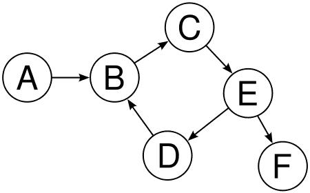
digraph
That is, the vertex set is $ \left \{ A,B,C,D,E,F \right \}$, the edge set (which is unlabeled in the picture) has size 6, and the adjacency function just formalizes which edges connect which vertices.
An undirected graph is a graph in which the edges are (for lack of a better word) undirected. There are two ways to realize this rigorously: one can view the codomain of the adjacency function $ \varphi$ as the set of subsets of size 2 of $ V$ as opposed to ordered pairs, or one can enforce that whenever $ \varphi(e) = (v_1, v_2)$ is a directed edge then so is $ (v_2, v_1)$. In our implementations we will stick to directed graphs, and our data structure will extend nicely to use the second definition if undirectedness is needed.
For the purpose of finding paths and simplicity in our derivations, we will impose two further conditions. First, the graphs must be simple. That is, no graph may have more than one edge between two vertices or self-adjacent vertices (that is, $ (v,v)$ can not be an edge for any vertex $ v$). Second, the graphs must be connected. That is, all pairs of vertices must have a path connecting them.
Our implementation of these algorithms will use a variation of the following Python data structure. This code should be relatively self-explanatory, but the beginning reader should consult our primers on the Python programming language for a more thorough explanation of classes and lists.
class Node:
   def __init__(self, value):
      self.value = value
      self.adjacentNodes = []
The entire graph will be accessible by having a reference to one vertex (this is guaranteed by connectivity). The vertex class is called Node, and it will contain as its data a value of arbitrary type and a list of neighboring vertices. For now the edges are just implicitly defined (there is an edge from $ v$ to $ w$ if the latter shows up in the “adjacentNodes” list of the former), but once we need edges with associated values we will have to improve this data structure to one similar to what we used in our post on neural networks.
That is, one must update the adjacentNodes attribute of each Node by hand to add edges to the graph. There are other data structures for graphs that allow one to refer to any vertex at any time, but for our purposes the constraint of not being able to do that is more enlightening. The algorithms we investigate will use no more and no less than what we have. At each stage we will inspect the vertex we currently have access to, and pick some action based on that.
Enough talk. Let’s jump right in!
Depth-First Search
For the remainder of this section, the goal is to determine if there is a vertex in the graph with the associated value being the integer 6. This can also be phrased more precisely as the question: “is there a path from the given node to a node with value 6?” (For connected. undirected graphs the two questions are equivalent.)
Our first algorithm will solve this problem quite nicely, and is called the depth-first search. Depth-first search is inherently a recursion:
- Start at a vertex.
- Pick any unvisited vertex adjacent to the current vertex, and check to see if this is the goal.
- If not, recursively apply the depth-first search to that vertex, ignoring any vertices that have already been visited.
- Repeat until all adjacent vertices have been visited.
This is probably the most natural algorithm in terms of descriptive simplicity. Indeed, in the case that our graph is a tree, this algorithm is precisely the preorder traversal.
Aside from keeping track of which nodes have already been visited, the algorithm is equally simple:
def depthFirst(node, soughtValue):
   if node.value == soughtValue:
      return True

   for adjNode in node.adjacentNodes:
      depthFirst(adjNode, soughtValue)
Of course, supposing 6 is not found, any graph which contains a cycle (or any nontrivial, connected, undirected graph) will cause this algorithm to loop infinitely. In addition, and this is a more subtle engineering problem, graphs with a large number of vertices will cause this function to crash by exceeding the maximum number of allowed nested function calls.
To avoid the first problem we can add an extra parameter to the function: a Python set type which contains the set of Nodes which have already been visited. Python sets are the computational analogue of mathematical sets, meaning that their contents are unordered and have no duplicates. And functionally Python sets have fast checks for inclusion and addition operations, so this fits the bill quite nicely.
The updated code is straightforward:
def depthFirst(node, soughtValue, visitedNodes):
   if node.value == soughtValue:
      return True

   visitedNodes.add(node)
   for adjNode in node.adjacentNodes:
      if adjNode not in visitedNodes:
         if depthFirst(adjNode, soughtValue, visitedNodes):
            return True

   return False
There are a few tricky things going on in this code snippet. First, after checking the current Node for the sought value, we add the current Node to the set of visitedNodes. While subsequently iterating over the adjacent Nodes we check to make sure the Node has not been visited before recursing. Since Python passes these sets by reference, changes made to visitedNodes deep in the recursion persist after the recursive call ends. That is, much the same as lists in Python, these updates mutate the object.
Second, this algorithm is not crystal clear on how the return values operate. Each recursive call returns True or False, but because there are arbitrarily many recursive calls made at each vertex, we can’t simply return the result of a recursive call. Instead, we can only know that we’re done entirely when a recursive call specifically returns True (hence the test for it in the if statement). Finally, after all recursive calls have terminated (and they’re all False), the end of the function defaults to returning False; in this case the sought vertex was never found.
Let’s try running our fixed code with some simple examples. In the following example, we have stored in the variable G the graph given in the picture in the previous section.
>>> depthFirst(G, "A")
True
>>> depthFirst(G, "E")
True
>>> depthFirst(G, "F")
True
>>> depthFirst(G, "X")
False
Of course, this still doesn’t fix the problem with too many recursive calls; a graph which is too large will cause an error because Python limits the number of recursive calls allowed. The next and final step is a standard method of turning a recursive algorithm into a non-recursive one, and it requires the knowledge of a particular data structure called a stack.
In the abstract, one might want a structure which stores a collection of items and has the following operations:
- You can quickly add something to the structure.
- You can quickly remove the most recently added item.
Such a data structure is called a stack. By “quickly,” we really mean that these operations are required to run in constant time with respect to the size of the list (it shouldn’t take longer to add an item to a long list than to a short one). One imagines a stack of pancakes, where you can either add a pancake to the top or remove one from the top; no matter how many times we remove pancakes, the one on top is always the one that was most recently added to the stack. These two operations are called push (to add) and pop (to remove). As a completely irrelevant aside, this is not the only algorithmic or mathematical concept based on pancakes.
In other languages, one might have to implement such a data structure by hand. Luckily for us, Python’s lists double as stacks (although in the future we plan some primers on data structure design). Specifically, the append function of a list is the push operation, and Python lists have a special operation uncoincidentally called pop which removes the last element from a list and returns it to the caller.
Here is some example code showing this in action:
>>> L = [1,2,3]
>>> L.append(9)
>>> L
[1,2,3,9]
>>> L.pop()
9
>>> L
[1,2,3]
Note that pop modifies the list and returns a value, while push/append only modifies the list.
It turns out that the order in which we visit the vertices in the recursive version of the depth-first search is the same as if we had done the following. At each vertex, push the adjacent vertices onto a stack in the reverse order that you iterate through the list. To choose which vertex to process next, simple pop whatever is on top of the stack, and process it (taking the stack with you as you go). Once again, we have to worry about which vertices have already been visited, and that part of the algorithm remains unchanged.
For example, say we have the following graph:
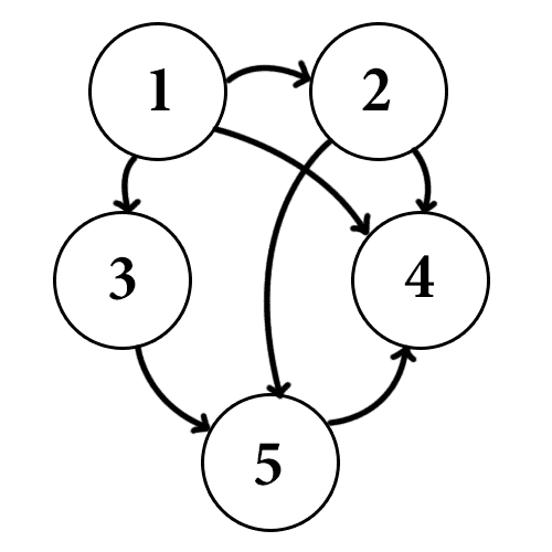
graph-dfs-stack-example1
Starting at vertex 1, which is adjacent to vertices 2, 3 and 4, we push 4 onto the stack, then 3, then 2. Next, we pop vertex 2 and iteratively process 2. At this point the picture looks like this:
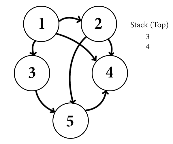
stack-example-two
Since 2 is connected to 4 and also 5, we push 5 and then 4 onto the stack. Note that 4 is in the stack twice (this is okay, since we are maintaining a set of visited vertices). Now the important part is that since we added vertex 5 and 4 after adding vertex 3, those will be processed before vertex 3. That is, the neighbors of more recently visited vertices (vertex 2) have a preference in being processed over the remaining neighbors of earlier ones (vertex 1). This is precisely the idea of recursion: we don’t finish the recursive call until all of the neighbors are processed, and that in turn requires the processing of all of the neighbors’ neighbors, and so on.
As a quick side note: it should be clear by now that the order in which we visit adjacent nodes is completely arbitrary in both versions of this algorithm. There is no inherent ordering on the edges of a vertex in a graph, and so adding them in reverse order is simply a way for us to mentally convince ourselves that the same preference rules apply with the stack as with recursion. That is, whatever order we visit them in the recursive version, we must push them onto the stack in the opposite order to get an identical algorithm. But in isolation neither algorithm requires a particular order. So henceforth, we will stop adding things in “reverse” order in the stack version.
Now the important part is that once we have converted the recursive algorithm into one based on a stack, we can remove the need for recursion entirely. Instead, we use a loop that terminates when the stack is empty:
def depthFirst(startingNode, soughtValue):
   visitedNodes = set()
   stack = [startingNode]

   while len(stack) > 0:
      node = stack.pop()
      if node in visitedNodes:
         continue

      visitedNodes.add(node)
      if node.value == soughtValue:
         return True

      for n in node.adjacentNodes:
         if n not in visitedNodes:
            stack.append(n)
   return False
This author particularly hates the use of “continue” in while loops, but its use here is better than any alternative this author can think of. For those unfamiliar: whenever a Python program encounters the continue statement in a loop, it skips the remainder of the body of the loop and begins the next iteration. One can also combine the last three lines of code into one using the lists’s extend function in combination with a list comprehension. This should be an easy exercise for the reader.
Moreover, note that this version of the algorithm removes the issue with the return values. It is quite easy to tell when we’ve found the required node or determined it is not in the graph: if the loop terminates naturally (that is, without hitting a return statement), then the sought value doesn’t exist.
The reliance of this algorithm on a data structure is not an uncommon thing. In fact, the next algorithm we will see cannot be easily represented as a recursive phenomenon; the order of traversal is simply too different. Instead, it will be almost identical to the stack-form of the depth-first search, but substituting a queue for a stack.
Breadth-First Search
As the name suggests, the breadth-first search operates in the “opposite” way from the depth-first search. Intuitively the breadth-first search prefers to visit the neighbors of earlier visited nodes before the neighbors of more recently visited ones. Let us reexamine the example we used in the depth-first search to see this change in action.
graph-dfs-stack-example1
Starting again with vertex 1, we add 4, 3, and 2 (in that order) to our data structure, but now we prefer the first thing added to our data structure instead of the last. That is, in the next step we visit vertex 4 instead of vertex 2. Since vertex 4 is adjacent to nobody, the recursion ends and we continue with vertex 3.
Now vertex 3 is adjacent to 5, so we add 5 to the data structure. At this point the state of the algorithm can be displayed like this:
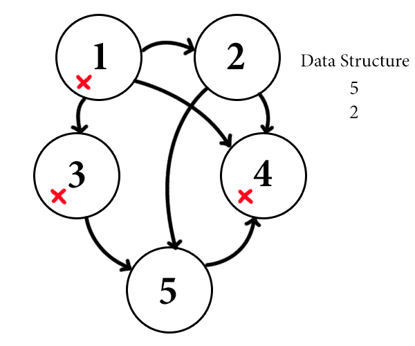
queue-example
That is, and this is the important bit, we process vertex 2 before we process vertex 5. Notice the pattern here: after processing vertex 1, we processed all of the neighbors of vertex 1 before processing any vertices not immediately adjacent to vertex one. This is where the “breadth” part distinguishes this algorithm from the “depth” part. Metaphorically, a breadth-first search algorithm will look all around a vertex before continuing on into the depths of a graph, while the depth-first search will dive straight to the bottom of the ocean before looking at where it is. Perhaps one way to characterize these algorithms is to call breadth-first cautious, and depth-first hasty. Indeed, there are more formal ways to make these words even more fitting that we will discuss in the future.
The way that we’ll make these rules rigorous is in the data-structure version of the algorithm: instead of using a stack we’ll use a queue. Again in the abstract, a queue is a data structure for which we’d like the following properties:
- We can quickly add items to the queue.
- We can quickly remove the least recently added item.
The operations on a queue are usually called enqueue (for additions) and dequeue (for removals).
Again, Python’s lists have operations that functionally make them queues, but the analogue of the enqueue operation is not efficient (specifically, it costs $ O(n)$ for a list of size $ n$). So instead we will use Python’s special deque class (pronounced “deck”). Deques are nice because they allow fast addition and removal from both “ends” of the structure. That is, deques specify a “left” end and a “right” end, and there are constant-time operations to add and remove from both the left and right ends.
Hence the enqueue operation we will use for a deque is called “appendleft,” and the dequeue operation is (unfortunately) called “pop.”
>>> from collections import deque
>>> queue = deque()
>>> queue.appendleft(7)
>>> queue.appendleft(4)
>>> queue
[4,7]
>>> queue.pop()
7
>>> queue
[4]
Note that a deque can also operate as a stack (it also has an append function with functions as the push operation). So in the following code for the breadth-first search, the only modification required to make it a depth-first search is to change the word “appendleft” to “append” (and to update the variable names from “queue” to “stack”).
And so the code for the breadth-first search algorithm is essentially identical:
from collections import deque

def breadthFirst(startingNode, soughtValue):
   visitedNodes = set()
   queue = deque([startingNode])

   while len(queue) > 0:
      node = queue.pop()
      if node in visitedNodes:
         continue

      visitedNodes.add(node)
      if node.value == soughtValue:
         return True

      for n in node.adjacentNodes:
         if n not in visitedNodes:
            queue.appendleft(n)
   return False
As in the depth-first search, one can combine the last three lines into one using the deque’s extendleft function.
We leave it to the reader to try some examples of running this algorithm (we repeated the example for the depth-first search in our code, but omit it for brevity).
Generalizing
After all of this exploration, it is clear that the depth-first search and the breadth-first search are truly the same algorithm. Indeed, the only difference is in the data structure, and this can be abstracted out of the entire procedure. Say that we have some data structure that has three operations: add, remove, and len (the Pythonic function for “query the size”). Then we can make a search algorithm that uses this structure without knowing how it works on the inside. Since words like stack, queue, and heap are already taken for specific data structures, we’ll call this arbitrary data structure a pile. The algorithm might look like the following in Python:
def search(startingNode, soughtValue, pile):
   visitedNodes = set()
   nodePile = pile()
   nodePile.add(startingNode)

   while len(nodePile) > 0:
      node = nodePile.remove()
      if node in visitedNodes:
         continue

      visitedNodes.add(node)
      if node.value == soughtValue:
         return True

      for n in node.adjacentNodes:
         if n not in visitedNodes:
            nodePile.add(n)
   return False
Note that the argument “pile” passed to this function is the constructor for the data type, and one of the first things we do is call it to create a new instance of the data structure for use in the rest of the function.
And now, if we wanted, we could recreate the depth-first search and breadth-first search as special cases of this algorithm. Unfortunately this would require us to add new methods to a deque, which is protected from such devious modifications by the Python runtime system. Instead, we can create a wrapper class as follows:
from collections import deque

class MyStack(deque):
   def add(self, item):
      self.append(item)

   def remove(self):
      return self.pop()

depthFirst = lambda node, val: search(node, val, MyStack)
And this clearly replicates the depth-first search algorithm. We leave the replication of the breadth-first algorithm as a trivial exercise (one need only modify two lines of the above code!).
It is natural to wonder what other kinds of magical data structures we could plug into this generic search algorithm. As it turns out, in the next post in this series we will investigate algorithms which do just that. The data structure we use will be much more complicated (a priority queue), and it will make use of additional information we assume away for this post. In particular, they will make informed decisions about which vertex to visit next at each step of the algorithm. We will also investigate some applications of these two algorithms next time, and hopefully we will see a good example of how they apply to artificial intelligence used in games.
Until then!
Want to respond? Send me an email, post a webmention, or find me elsewhere on the internet.