The Problem with Cropping
Every programmer or graphic designer with some web development experience can attest to the fact that finding good images that have an exactly specified size is a pain. Since the dimensions of the sought picture are usually inflexible, an uncomfortable compromise can come in the form of cropping a large image down to size or scaling the image to have appropriate dimensions.
Both of these solutions are undesirable. In the example below, the caterpillar looks distorted in the scaled versions (top right and bottom left), and in the cropped version (bottom right) it’s more difficult to tell that the caterpillar is on a leaf; we have lost the surrounding context.
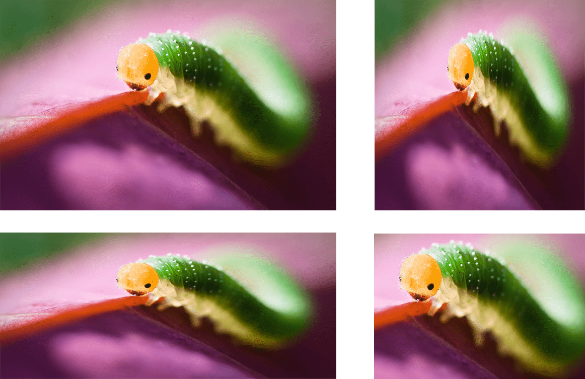
scaling-gone-wrong
In this post we’ll look at a nice heuristic method for rescaling images called seam-carving, which pays attention to the contents of the image as it resacles. In particular, it only removes or adds pixels to the image that the viewer is least-likely to notice. In all but the most extreme cases it will avoid the ugly artifacts introduced by cropping and scaling, and with a bit of additional scaffolding it becomes a very useful addition to a graphic designer’s repertoire. At first we will focus on scaling an image down, and then we will see that the same technique can be used to enlarge an image.
Before we begin, we should motivate the reader with some examples of its use.
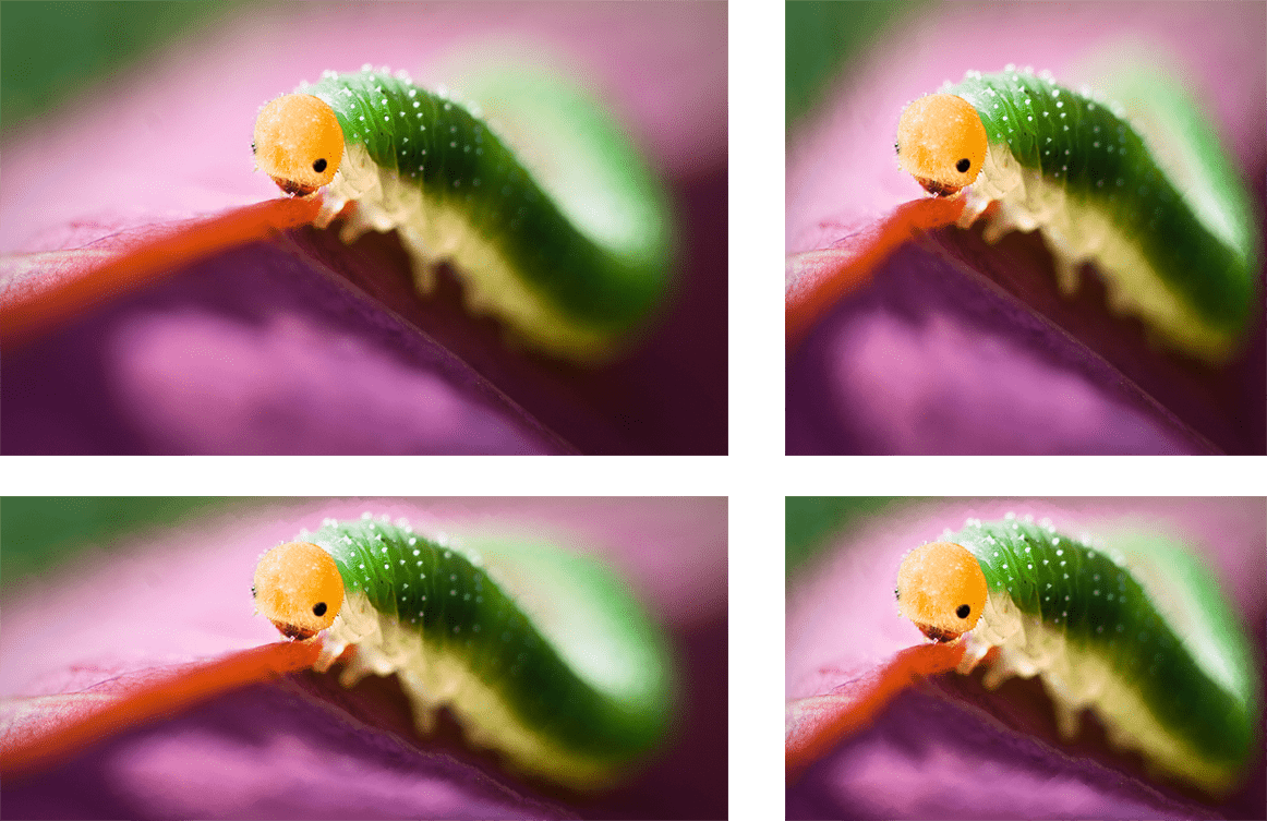
example-seam-carving
It’s clear that the caterpillar is far less distorted in all versions, and even in the harshly rescaled version, parts of the green background are preserved. Although the leaf is warped a little, it is still present, and it’s not obvious that the image was manipulated.
Now that the reader’s appetite has been whet, let’s jump into the mathematics of it. This method was pioneered by Avidan and Shamir, and the impatient reader can jump straight to their paper (which contains many more examples). In this post we hope to fill in the background and show a working implementation.
Images as Functions
One common way to view an image is as an approximation to a function of two real variables. Suppose we have an $ n \times m$-pixel image ($ n$ rows and $ m$ columns of pixels). For simplicity (during the next few paragraphs), we will also assume that the pixel values of an image are grayscale intensity values between 0 and 255. Then we can imagine the pixel values as known integer values of a function $ f: \mathbb{R}^n \times \mathbb{R}^m \to \mathbb{R}$. That is, if we take two integers $ 0 \leq x < n$ and $ 0 \leq y < m$ then we know the value $ f(x,y)$; it’s just the intensity value at the corresponding pixel. For values outside these ranges, we can impose arbitrary values for $ I$ (we don’t care what’s happening outside the image).
Moreover, it makes sense to assume that $ f$ is a well-behaved function in between the pixels (i.e. it is differentiable). And so we can make reasonable guessed as to the true derivative of $ f$ by looking at the differences between adjacent pixels. There are many ways to get a good approximation of the derivative of an image function, but we should pause a moment to realize why this is important to nail down for the purpose of resizing images.
A good rule of thumb with images is that regions of an image which are most important to the viewer are those which contain drastic changes in intensity or color. For instance, consider this portrait of Albert Einstein.

Which parts of this image first catch the eye? The unkempt hair, the wrinkled eyes, the bushy mustache? Certainly not the misty background, or the subtle shadows on his chin.
Indeed, one could even claim that an image having a large derivative at a certain pixel corresponds to high information content there (of course this is not true of all images, but perhaps it’s reasonable to claim this for photographs). And if we want to scale an image down in size, we are interested in eliminating those regions which have the smallest information content. Of course we cannot avoid losing some information: the image after resizing is smaller than the original, and a reasonable algorithm should not add any new information. But we can minimize the damage by intelligently picking which parts to remove; our naive assumption is that a small derivative at a pixel implies a small amount of information.
Of course we can’t just remove “regions” of an image to change its proportions. We have to remove the same number of pixels in each row or column to reduce the corresponding dimension (width or height, resp.). Before we get to that, though, let’s write a program to compute the gradient. For this program and the rest of the post we will use the Processing programming language, and our demonstrations will use the Javascript cross-compiler processing.js. The nice thing about Processing is that if you know Java then you know processing. All the basic language features are the same, and it’s just got an extra few native types and libraries to make graphics rendering and image displaying easier. As usual, all of the code used in this blog post is available on this blog’s Github page.
Let’s compute the gradient of this picture, and call the picture $ I$:

A very nice picture whose gradient we can compute. It was taken by the artist [Ria Czichotzki](https://www.rialeephotography.com/).
Since this is a color image, we will call it a function $ I: \mathbb{R}^2 \to \mathbb{R}^3$, in the sense that the input is a plane coordinate $ (x,y)$, and the output $ I(x,y) = (r,g,b)$ is a triple of color intensity values. We will approximate the image’s partial derivative $ \left \langle \partial I / \partial x, \partial I / \partial y \right \rangle$ at $ (x,y)$ by inspecting values of $ I$ in a neighborhood of the point:
$ I(x-1,y), I(x+1, y), I(x,y-1), I(x,y+1)$.
For each pixel we call the value $ |I(x+1,y) – I(x-1,y)| / 2$ the partial derivative in the $ x$ direction, and $ |I(x,y+1) – I(x,y-1)| / 2$ the partial in the $ y$ direction. Note that the values $ I(x,y)$ are vectors, so the norm signs here are really computing the distance between the two values of $ I$.
There are two ways to see why this makes sense as an approximation. The first is analytic: by definition, the partial derivative $ \partial I / \partial x$ is a limit:
$$\displaystyle \lim_{h \to 0} \frac{|I(x+h,y) – I(x,y)|}{h}$$It turns out that this limit is equivalent to
$$\displaystyle \lim_{h \to 0} \frac{|I(x+h,y) – I(x-h,y)|}{2h}$$And the closer $ h$ gets to zero the better the approximation of the limit is. Since the closest we can make $ h$ is $ h=1$ (we don’t know any other values of $ I$ with nonzero $ h$), we plug in the corresponding values for neighboring pixels. The partial $ \partial I / \partial y$ is similar.
The second way to view it is geometric.
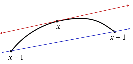
The slope of the blue secant line is not a bad approximation to the derivative at x, provided the resolution is fine enough.
The salient fact here is that a nicely-behaved curve at $ x$ will have a derivative close to the secant line between the points $ (x-1, f(x-1))$ and $ (x+1, f(x+1))$. Indeed, this idea inspires the original definition of the derivative. The slope of the secant line is just $ (f(x+1) – f(x-1)) / 2$. As we saw in our post on numerical integration, we can do much better than a linear guess (specifically, we can use do any order of polynomial interpolation we wish), but for the purposes of displaying the concept of seam-carving, a linear guess will suffice.
And so with this intuitive understanding of how to approximate the gradient, the algorithm to actually do it is a straightforward loop. Here we compute the horizontal gradient (that is, the derivative $ \partial I / \partial x$).
PImage horizontalGradient(PImage img) {
   color left, right;
   int center;
   PImage newImage = createImage(img.width, img.height, RGB);

   for (int x = 0; x < img.width; x++) {
      for (int y = 0; y < img.height; y++) {
         center = x + y*img.width;

         left = x == 0 ? img.pixels[center] : img.pixels[(x-1) + y*img.width];
         right = x == img.width-1 ? img.pixels[center] : img.pixels[(x+1) + y*img.width];

         newImage.pixels[center] = color(colorDistance(left, right));
      }
   }

   return newImage;
}
The details are a bit nit-picky, but the idea is simple. If we’re inspecting a non-edge pixel, then we can use the formula directly and compute the values of the neighboring left and right pixels. Otherwise, the “left” pixel or the “right” pixel will be outside the bounds of the image, and so we replace it with the pixel we’re inspecting. Mathematically, we’d be computing the difference $ |I(x, y) – I(x+1, y)|$ and $ |I(x-1,y) – I(x, y)|$. Additionally, since we’ll later only be interested in the relative sizes of the gradient, we can ignore the factor of 1/2 in the formula we derived.
The parts of this code that are specific to Processing also deserve some attention. Specifically, we use the built-in types PImage and color, for representing images and colors, respectively. The “createImage” function creates an empty image of the specified size. And peculiarly, the pixels of a PImage are stored as a one-dimensional array. So as we’re iterating through the rows and columns, we must compute the correct location of the sought pixel in the pixel array (this is why we have a variable called “center”). Finally, as in Java, the ternary if notation is used to keep the syntax short, and those two lines simply check for the boundary conditions we stated above.
The last unexplained bit of the above code is the “colorDistance” function. As our image function $ I(x,y)$ has triples of numbers as values, we need to compute the distance between two values via the standard distance formula. We have encapsulated this in a separate function. Note that because (in this section of the blog) we are displaying the results in an image, we have to convert to an integer at the end.
int colorDistance(color c1, color c2) {
   float r = red(c1) - red(c2);
   float g = green(c1) - green(c2);
   float b = blue(c1) - blue(c2);
   return (int)sqrt(r*r + g*g + b*b);
}
Let’s see this in action on the picture we introduced earlier.

gradient-girl
The reader who is interested in comparing the two more closely may visit this interactive page. Note that we only compute the horizontal gradient, so certain locations in the image have a large derivative but are still dark in this image. For instance, the top of the door in the background and the wooden bars supporting the bottom of the chair are dark despite the vertical color variations.
The vertical gradient computation is entirely analogous, and is left as an exercise to the reader.
Since we want to inspect both vertical and horizontal gradients, we will call the total gradient matrix $ G$ the matrix whose entries $ g_{i,j}$ are the sums of the magnitudes of the horizontal and vertical gradients at $ i,j$:
$$\displaystyle g_{i,j} = \left | \frac{\partial I}{\partial x} (i,j) \right | + \left | \frac{\partial I}{\partial y} (i,j) \right |$$The function $ e(x,y) = g_{x,y}$ is often called an energy function for $ I$. We will mention now that there are other energy functions one can consider, and use this energy function for the remainder of this post.
Seams, and Dynamic Programming
Back to the problem of resizing, we want a way to remove only those regions of an image that have low total gradient across all of the pixels in the region removed. But of course when resizing an image we must maintain the rectangular shape, and so we have to add or remove the same number of pixels in each column or row.
For the purpose of scaling an image down in width (and the other cases are similar), we have a few options. We could find the pixel in each row with minimal total gradient and remove it. More conservatively, we could remove those columns with minimal gradient (as a sum of the total gradient of each pixel in the column). More brashly, we could just remove pixels of lowest gradient willy-nilly from the image, and slide the rows left.
If none of these ideas sound like they would work, it’s because they don’t. We encourage the unpersuaded reader to try out each possibility on a variety of images to see just how poorly they perform. But of these options, removing an entire column happens to distort the image less than the others. Indeed, the idea of a “seam” in an image is just a slight generalization of a column. Intuitively, a seam $ s_i$ is a trail of pixels traversing the image from the bottom to the top, and at each step the pixel trail can veer to the right or left by at most one pixel.
Definition: Let $ I$ be an $ n \times m$ image with nonnegative integer coordinates indexed from zero. A vertical seam in $ I$ is a list of coordinates $ s_i = (x_i, y_i)$ with the following properties:
- $ y_0 = 0$ is at the bottom of the image.
- $ y_{n-1} = n-1$ is at the top of the image.
- $ y_i$ is strictly increasing.
- $ |x_i – x_{i+1}| \leq 1$ for all $ 0 \leq i < n-1$.
These conditions simply formalize what we mean by a seam. The first and second impose that the seam traverses from top to bottom. The third requires the seam to always “go up,” so that there is only one pixel in each row. The last requires the seam to be “connected” in the sense that it doesn’t veer too far at any given step.
Here are some examples of some vertical seams. One can easily define horizontal seams by swapping the placement of $ x, y$ in the above list of conditions.
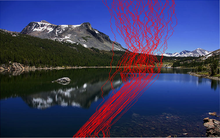
glacier_canyon_h_shr_seams
So the goal is now to remove the seams of lowest total gradient. Here the total gradient of a seam is just the sum of the energy values of the pixels in the seam.
Unfortunately there are many more seams to choose from than columns (or even individual pixels). It might seem difficult at first to find the seam with the minimal total gradient. Luckily, if we’re only interested in minima, we can use dynamic programming to compute the minimal seam ending at any given pixel in linear time.
We point the reader unfamiliar with dynamic programming to our Python primer on this topic. In this case, the sub-problem we’re working with is the minimal total gradient value of all seams from the bottom of the image to a fixed pixel. Let’s call this value $ v(a,b)$. If we know $ v(a,b)$ for all pixels below, say, row $ i$, then we can compute the $ v(i+1,b)$ for the entire row $ i+1$ by taking pixel $ (i+1,j)$, and adding its gradient value to the minimum of the values of possible predecessors in a seam, $ v(i,j-1), v(i,j), v(i,j+1)$ (respecting the appropriate boundary conditions).
Once we’ve computed $ v(a,b)$ for the entire matrix, we can look at the minimal value at the top of the image $ \min_j v(n,j)$, and work backwards down the image to compute which seam gave us this minimum.
Let’s make this concrete and compute the function $ v$ as a two-dimensional array called “seamFitness.”
void computeVerticalSeams() {
   seamFitness = new float[img.width][img.height];
   for (int i = 0; i < img.width; i++) {
      seamFitness[i][0] = gradientMagnitude[i][0];
   }

   for (int y = 1; y < img.height; y++) {
      for (int x = 0; x < img.width; x++) {
         seamFitness[x][y] = gradientMagnitude[x][y];

         if (x == 0) {
            seamFitness[x][y] += min(seamFitness[x][y-1], seamFitness[x+1][y-1]);
         } else if (x == img.width-1) {
            seamFitness[x][y] += min(seamFitness[x][y-1], seamFitness[x-1][y-1]);
         } else {
            seamFitness[x][y] += min(seamFitness[x-1][y-1], seamFitness[x][y-1], seamFitness[x+1][y-1]);
         }
      }
   }
}
We have two global variables at work here (global is bad, I know, but it’s Processing; it’s made for prototyping). The seamFitness array, and the gradientMagnitude array. We assume at the start of this function that the gradientMagnitude array is filled with sensible values.
Here we first initialize the zero’th row of the seamFitness array to have the same values as the gradient of the image. This is simply because a seam of length 1 has only one gradient value. Note here the coordinates are a bit backwards: the first coordinate represents the choice of a column, and the second represents the choice of a row. We can think of the coordinate axes of our image function having the origin in the bottom-left, the same as we might do mathematically.
Then we iterate over the rows in the matrix, and in each column we compute the fitness based on the fitness of the previous row. That’s it 🙂
To actually remove a seam, we need to create a new image of the right size, and shift the pixels to the right (or left) of the image into place. The details are technically important, but tedious to describe fully. So we leave the inspection of the code as an exercise to the reader. We provide the Processing code on this blog’s Github page, and show an example of its use below. Note each the image resizes every time the user clicks within the image.
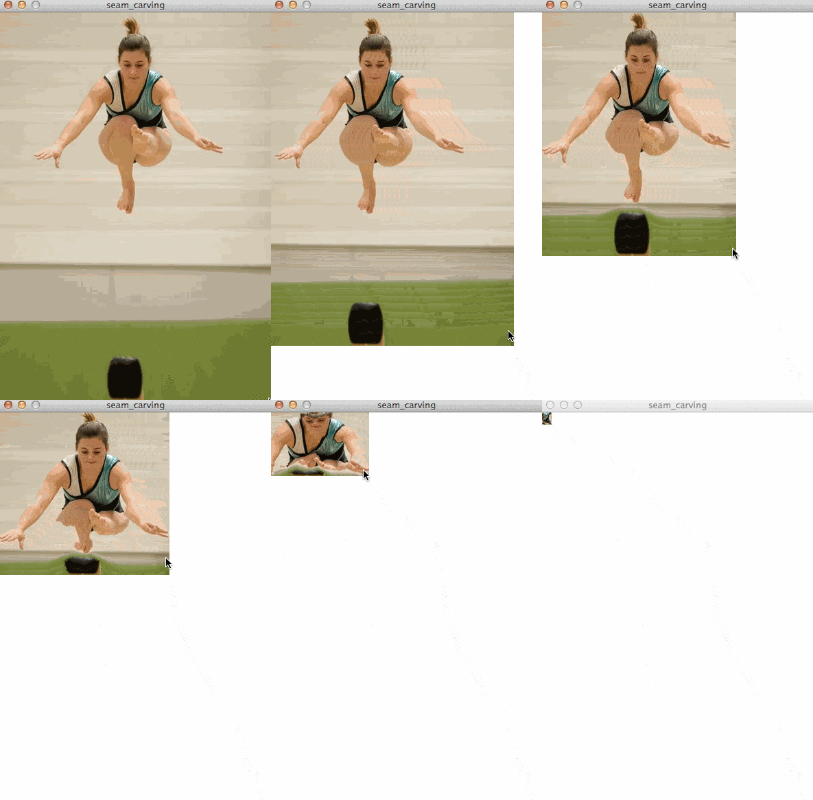
seam-carving-demo
It’s interesting (and indeed the goal) to see how at first nothing is warped, and then the lines on the walls curve around the woman’s foot, and then finally the woman’s body is distorted before she gets smushed into a tiny box by the oppressive mouse.
As a quick side note, we attempted to provide an interactive version of this Processing program online in the same way we did for the gradient computation example. Processing is quite nice in that any Processing program (which doesn’t use any fancy Java libraries) can be cross-compiled to Javascript via the processing.js library. This is what we did for the gradient example. But in doing so for the (admittedly inefficient and memory-leaky) seam-carving program, it appeared to run an order of magnitude slower in the browser than locally. This was this author’s first time using Processing, so the reason for the drastic jump in runtime is unclear. If any readers are familiar with processing.js, a clarification would be very welcome in the comments.
Inserting Seams, Removing Objects, and Videos
In addition to removing seams to scale an image down, one can just as easily insert seams to make an image larger. To insert a seam, just double each pixel in the seam and push the rest of the pixels on the row to the right. The process is not hard, but it requires avoiding one pitfall: if we just add a single seam at a time, then the seam with minimum total energy will never change! So we’ll just add the same seam over and over again. Instead, if we want to add $ k$ seams, one should compute the minimum $ k$ seams and insert them all. If the desired resize is too large, then the programmer should pick an appropriate batch size and add seams in batches.
Another nice technique that comes from the seam-carving algorithm is to intelligently protect or destroy specific regions in the image. To do this requires a minor modification of the gradient computation, but the rest of the algorithm is identical. To protect a region, provide some way of user input specifying which pixels in the image are important, and give those pixels an artificially large gradient value (e.g., the maximum value of an integer). If the down-scaling is not too extreme, the seam computations will be guaranteed not to use any of those pixels, and inserted seams will never repeat those pixels. To remove a region, we just give the desired pixels an arbitrarily low gradient value. Then these pixels will be guaranteed to occur in the minimal seams, and will be removed from the picture.
The technique of seam-carving is a very nice tool, and as we just saw it can be extended to a variety of other techniques. In fact, seam-carving and its applications to object removal and image resizing are implemented in all of the recent versions of Photoshop. The techniques are used to adapt applications to environments with limited screen space, such as a mobile phone or tablet. Seam carving can even be adapted for use in videos. This involves an extension of the dynamic program to work across multiple frames, formally finding a minimal graph cut between two frames so that each piece of the cut is a seam in the corresponding frame. Of course there is a lot more detail to it (and the paper linked above uses this detail to improve the basic image-resizing algorithm), but that’s the rough idea.
We’ve done precious little on this blog with images, but we’d like to get more into graphics programming. There’s a wealth of linear algebra, computational geometry, and artificial intelligence hiding behind most of the computer games we like to play, and it would be fun to dive deeper into these topics. Of course, with every new post this author suggests ten new directions for this blog to go. It’s a curse and a blessing.
Until next time!
Want to respond? Send me an email, post a webmention, or find me elsewhere on the internet.