One of the main areas of difficulty in elementary probability, and one that requires the highest levels of scrutiny and rigor, is conditional probability. The ideas are simple enough: that we assign probabilities relative to the occurrence of some event. But shrewd applications of conditional probability (and in particular, efficient ways to compute conditional probability) are key to successful applications of this subject. This is the basis for Nate Silver‘s success, the logical flaws of many a political pundit, and the ability for a robot to tell where it is in an environment. As this author usually touts, the best way to avoid the pitfalls of such confusing subjects is to be mathematically rigorous. In doing so we will develop intuition for when conditional probability that experts show off as if it were trivial.
But before we can get to all of that, we will cover a few extra ideas from finite probability theory that were left out of the last post.
Our entire discussion will revolve around a finite probability space, as defined last time. Let’s briefly (and densely) recall some of the notation presented there. We will always denote our probability space by $ \Omega$, and the corresponding probability mass function will be $ f: \Omega \to [0,1]$. Recall that events are subsets $ E \subset \Omega$, and the probability function $ P$ accepts as inputs events $ E$, and produces as output the sum of the probabilities of members of $ E$. We abuse notation by saying $ \textup{P}(x) = \textup{P}(\left \{ x \right \}) = f(x)$ and disregarding $ f$ for the most part. We really think of $ \textup{P}$ as an extension of $ f$ to subsets of $ \Omega$ instead of just single values of $ \Omega$. Further recall that a random variable $ X$ is a real-valued function function $ \Omega \to \mathbb{R}$.
Partitions and Total Probability
A lot of reasoning in probability theory involves decomposing a complicated event into simpler events, or decomposing complicated random variables into simpler ones. Conditional probability is one way to do that, and conditional probability has very nice philosophical interpretations, but it fits into this more general scheme of “decomposing” events and variables into components.
The usual way to break up a set into pieces is via a partition. Recall the following set-theoretic definition.
Definition: A partition of a set $ X$ is a collection of subsets $ X_i \in X$ so that every element $ x \in X$ occurs in exactly one of the $ X_i$.
Here are a few examples. We can partition the natural numbers $ \mathbb{N}$ into even and odd numbers. We can partition the set of people in the world into subsets where each subset corresponds to a country and a person is placed in the subset corresponding to where they were born (an obvious simplification of the real world, but illustrates the point). The avid reader of this blog will remember how we used partitions to define quotient groups and quotient spaces. With a more applied flavor, finding a “good” partition is the ultimate goal of the clustering problem, and we saw a heuristic approach to this in our post on Lloyd’s algorithm.

You should think of a partition as a way to “cut up” a set into pieces. This colorful diagram is an example of a partition of a disc.
In fact, any time we have a canonical way to associate two things in a set, we can create a partition by putting all mutually associated things in the same piece of the partition. The rigorous name for this is an equivalence relation, but we won’t need that for the present discussion (partitions are the same thing as equivalence relations, just viewed in a different way).
Of course, the point is to apply this idea to probability spaces. Points (elements) in our probability space $ \Omega$ are outcomes of some random experiment, and subsets $ E \subset \Omega$ are events. So we can rephrase a partition for probability spaces as a choice of events $ E_i \subset \Omega$ so that every outcome in $ \Omega$ is part of exactly one event. Our first observation is quite a trivial one: the probabilities of the events in a partition sum to one. In symbols, if $ E_1, \dots, E_m$ form our partition, then
$$\displaystyle \sum_{i=1}^m \textup{P}(E_i) = 1$$Indeed, the definition of $ \textup{P}$ is to sum over the probabilities of outcomes in an event. Since each outcome occurs exactly once among all the $ E_i$, the above sum expands to
$$\displaystyle \sum_{\omega \in \Omega} \textup{P}(\omega)$$Which by our axioms for a probability space is just one. We will give this observation the (non-standard) name the Lemma of Total Probability.
This was a nice warmup proof, but we can beef it up to make it more useful. If we have some other event $ A$ which is not related to a partition in any way, we can break up $ A$ with respect to the partition. Then, assuming this is simpler, we compute the probability that $ A$ happens in terms of the probabilities of the pieces.
Theorem: Let $ E_1, \dots , E_m$ be a partition of $ \Omega$, and let $ A$ be an arbitrary event. Then
$$\displaystyle \textup{P}(A) = \sum_{i=1}^m \textup{P}(E_i \cap A)$$Proof. The proof is only marginally more complicated than that of the lemma of total probability. The probability of the event $ A$ occurring is the sum of the probabilities of each of its outcomes occurring. Each outcome in $ A$ occurs in exactly one of the $ E_i$, and hence in exactly one of the sets $ E_i \cap A$. If $ E_i \cap A$ is empty, then its probability of occurring is zero (as per our definitions last time). So the sum on the right expands directly into the definition of $ \textup{P}(A)$. $ \square$
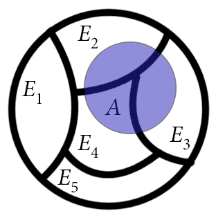
The area taken up by the set A is the same as the area taken up by the pieces of A which overlap the E's
A more useful way of thinking of this is that we can use the $ E_i$ to define a partition of $ A$ in a natural way. The subsets in the partition will just be the sets $ E_i \cap A$, and we will throw out any of these that turn out to be empty. Then we can think of our “new” probability space being $ A$, and the theorem is just a special case of the lemma of total probability. Interestingly enough, this special case is often called the Theorem of Total Probability.
The idea to think of the event $ A$ as our “new” probability space is extremely useful. It shows its worth most prominently when we interpret the shift as, “gaining the information that $ A$ has occurred.” Then the question becomes: given that $ A$ occurs, what is the probability that some other event will occur? That is, we’re interested in the probability of some event $ B$ relative to $ A$. This is called the conditional probability of $ B$ with respect to $ A$, and is denoted $ P(B | A)$ (read “the probability of B given A”).
To compute the conditional probability, simply scale $ \textup{P}(A \cap B)$ by the assumed event $ \textup{P}(A)$. That is,
$$\displaystyle \textup{P}(B | A) = \frac{\textup{P}(A \cap B)}{\textup{P}(A)}$$Wikipedia provides a straightforward derivation of the formula, but the spirit of the proof is exactly what we said above. The denominator is our new sample space, and the numerator is the probability of outcomes that cause $ B$ to occur which also cause $ A$ to occur. Multiplying both sides of this formula by $ \textup{P}(A)$, this identity can be used to arrive at another version of the theorem of total probability:
$ \displaystyle \textup{P}(A) = \sum_{i=1}^m \textup{P}(A | E_i) \textup{P}(E_i)$
That is, if we know how to compute the probabilities of the $ E_i$, and we know how likely $ A$ is to occur in each of those scenarios, then we can compute the total probability of $ A$ occurring independently of the $ E_i$.
We can come up with loads of more or less trivial examples of the theorem of total probability on simple probability spaces. Say you play a craps-like game where you roll a die twice. If you get a one on the first roll, you lose, and otherwise you have to match your initial roll on the second to win. The probability you win can be analyzed with the theorem on total probability. We partition the sample space into events corresponding to the outcome of the first roll.
$$\displaystyle \textup{P}(\textup{Win}) = \sum_{i=1}^6 \textup{P}(\textup{Win } | \textup{ 1st roll }= i) \textup{P}(\textup{1st roll } = i)$$The probability the first roll is $ i$ is 1/6, and if the first roll is a 1 then the probability of winning after that is zero. In the other 5 cases the conditional probability is the same regardless of $ i$: to match $ i$ on the second roll has a 1/6 chance. So the probability of winning is
$$\displaystyle 5 \cdot \frac{1}{6} \cdot \frac{1}{6} = \frac{5}{36}$$For the working mathematician, these kinds of examples are relatively low-tech, but it illustrates the main way conditional probability is used in practice. We have some process we want to analyze, and we break it up into steps and condition on the results of a given step. We will see in a moment a more complicated example of this.
Partitions via Random Variables
The most common kind of partition is created via a random variable with finitely many values (or countably many, but we haven’t breached infinite probability spaces yet). In this case, we can partition the sample space $ \Omega$ based on the values of $ X$. That is, for each value $ x = X(\omega)$, we will have a subset of the partition $ S_x$ be the set of all $ \omega$ which map to $ x$. In the parlance of functions, it is the preimage of a single value $ x$;
$$\displaystyle S_x = X^{-1}(x) = \left \{ \omega \in \Omega : X(\omega) = x\right \}$$And as the reader is probably expecting, we can use this to define a “relative” expected value of a random variable. Recall that if the image of $ X$ is a finite set $ x_1, \dots, x_n$, the expected value of $ X$ is a sum
$$\displaystyle \textup{E}(X) = \sum_{i=1}^n x_i \textup{P}(X = x_i)$$Suppose $ X,Y$ are two such random variables, then the conditional probability of $ X$ relative to the event $ Y=y$ is the quantity
$$\displaystyle \textup{P}(X=x | Y=y) = \frac{\textup{P}(X=x \textup{ and } Y=y)}{\textup{P}(Y=y)}$$And the conditional expectation of $ X$ relative to the event $ Y = y$, denoted $ \textup{E}(X | Y = y)$ is a similar sum
$$\displaystyle \textup{E}(X|Y=y) = \sum_{i=1}^n x_i \textup{P}(X = x_i | Y = y)$$Indeed, just as we implicitly “defined” a new sample space when we were partitioning based on events, here we are defining a new random variable (with the odd notation $ X | Y=y$) whose domain is the preimage $ Y^{-1}(y)$. We can then ask what the probability of it assuming a value $ x$ is, and moreover what its expected value is.
Of course there is an analogue to the theorem of total probability lurking here. We want to say something like the true expected value of $ X$ is a sum of the conditional expectations over all possible values of $ Y$. We have to remember, though, that different values of $ y$ can occur with very different probabilities, and the expected values of $ X | Y=y$ can change wildly between them. Just as a quick (and morbid) example, if $ X$ is the number of people who die on a randomly chosen day, and $ Y$ is the number of atomic bombs dropped on that day, it is clear that the probability of $ Y$ being positive is quite small, and the expected value of $ X = Y=y$ will be dramatically larger if $ y$ is positive than if it’s zero. (A few quick calculations based on tragic historic events show it would roughly double, using contemporary non-violent death rate estimates.)
And so instead of simply summing the expectation, we need to take an expectation over the values of $ Y$. Thinking again of $ X | Y=y$ as a random variable based on values of $ Y$, it makes sense mathematically to take expectation. To distinguish between the two types of expectation, we will subscript the variable being “expected,” as in $ \textup{E}_X(X|Y)$. That is, we have the following theorem.
Theorem: The expected value of $ X$ satisfies
$$\textup{E}_X(X) = \textup{E}_Y(\textup{E}_X(X|Y))$$Proof. Expand the definitions of what these values mean, and use the definition of conditional probability $ \textup{P}(A \cap B) = \textup{P}(A | B) \textup{P}(B)$. We leave the proof as a trivial exercise to the reader, but if one cannot bear it, see Wikipedia for a full proof. $ \square$
Let’s wrap up this post with a non-trivial example of all of this theory in action.
A Nontrivial Example: the Galton-Watson Branching Process
We are interested (as was the eponymous Sir Francis Galton in the 1800’s) in the survival of surnames through generations of marriage and children. The main tool to study such a generational phenomenon is the Galton-Watson branching process. The idea is quite simple, but its analysis quickly blossoms into a rich and detailed theoretical puzzle and a more general practical tool. Just before we get too deep into things, we should note that these ideas (along with other types of branching processes) are used to analyze a whole host of problems in probability theory and computer science. A few the author has recently been working with are the evolution of random graphs and graph property testing.
The gist is as follows: say we live in a patriarchal society in which surnames are passed down on the male side. We can image a family tree being grown step by step in this way At the root there is a single male, and he has $ k$ children, some of which are girls and some of which are boys. They all go on to have some number of children, but only the men pass on the family name to their children, and only their male children pass on the family name further. If we only record the family tree along the male lines, we can ask whether the tree will be finite; that is, whether the family name will die out.
To make this rigorous, let us define an infinite sequence of random variables $ X_1 X_2, \dots$ which represent the number of children each person in the tree has, and suppose further that all of these variables are independent and uniformly distributed from $ 1, \dots, n$ for some fixed $ n$. This may be an unrealistic assumption, but it makes the analysis a bit simpler. The number of children more likely follows a Poisson distribution where the mean is a parameter we would estimate from real-world data, but we haven’t spoken of Poisson distributions on this blog yet so we will leave it out.
We further imagine the tree growing step by step: at step $ i$ the $ i$-th individual in the tree has $ X_i$ children and then dies. If the individual is a woman we by default set $ X_i = 0$. We can recursively describe the size of the tree at each step by another random variable $ Y_i$. Clearly $ Y_0 = 1$, and the recursion is $ Y_n = Y_{n-1} + X_i – 1$. In words, $ Y_i$ represents the current living population with the given surname. We say the tree is finite (the family name dies off), if for some $ i$ we get $ Y_i = 0$. The first time at which this happens is when the family name dies off, but abstractly we can imagine the sequence of random variables continuing forever. This is sometimes called fictitious continuation.
At last, we assume that the probability of having a boy or girl is a split 1/2. Now we can start asking questions. What is the probability that the surname dies off? What is the expected size of the tree in terms of $ n$?
For the first question we use the theorem of total probability. In particular, suppose the first person has two boys. Then the whole tree is finite precisely when both boys’ sub-trees are finite. Indeed, the two boys’ sub-trees are independent of one another, and so the probability of both being finite is the product of the probabilities of each being finite. That is, more generally
$$\displaystyle \textup{P}(\textup{finite } | k \textup{ boys}) = \textup{P}(\textup{finite})^k \textup{P}(\textup{two boys})$$Setting $ z = \textup{P}(\textup{the tree is finite})$, we can compute $ z$ directly by conditioning on all possibilities of the first person’s children. Notice how we must condition twice here.
$$\displaystyle z = \sum_{i=0}^n \sum_{k=0}^i \textup{P}(k \textup{ boys } | i \textup{ children}) \textup{P}(i \textup{ children}) z^k$$The probability of getting $ k$ boys is the same as flipping $ i$ coins and getting $ k$ heads, which is just
$$\displaystyle \textup{P}(k \textup{ boys } | i \textup{ children}) = \binom{i}{k}\frac{1}{2^i}$$So the equation is
$$\displaystyle z = \sum_{i=0}^n \sum_{k=0}^i \binom{i}{k} \frac{1}{2^i} \cdot \frac{1}{n} z^k$$From here, we’ve reduced the problem down to picking the correct root of a polynomial. For example, when $ n=4$, the polynomial equation to solve is
$$\displaystyle 64z = 5 + 10z + 10z^2 + 5z^3 + z^4$$We have to be a bit careful, here though. Not all solutions to this equation are valid answers. For instance, the roots must be between 0 and 1 (inclusive), and if there are multiple then one must rule out the irrelevant roots by some additional argument. Moreover, we would need to use a calculus argument to prove there is always a solution between 0 and 1 in the first place. But after all that is done, we can estimate the correct root computationally (or solve for exactly when our polynomials have small degree). Here for $ n=4$, the probability of being finite is about 0.094.
We leave the second question, on the expected size of the tree, for the reader to ponder. Next time we’ll devote an entire post to Bayes Theorem (a trivial consequence of the definition of conditional probability), and see how it helps us compute probabilities for use in programs.
Until then!
Want to respond? Send me an email, post a webmention, or find me elsewhere on the internet.