This series on topology has been long and hard, but we’re are quickly approaching the topics where we can actually write programs. For this and the next post on homology, the most important background we will need is a solid foundation in linear algebra, specifically in row-reducing matrices (and the interpretation of row-reduction as a change of basis of a linear operator).
Last time we engaged in a whirlwind tour of the fundamental group and homotopy theory. And we mean “whirlwind” as it sounds; it was all over the place in terms of organization. The most important fact that one should take away from that discussion is the idea that we can compute, algebraically, some qualitative features about a topological space related to “n-dimensional holes.” For one-dimensional things, a hole would look like a circle, and for two dimensional things, it would look like a hollow sphere, etc. More importantly, we saw that this algebraic data, which we called the fundamental group, is a topological invariant. That is, if two topological spaces have different fundamental groups, then they are “fundamentally” different under the topological lens (they are not homeomorphic, and not even homotopy equivalent).
Unfortunately the main difficulty of homotopy theory (and part of what makes it so interesting) is that these “holes” interact with each other in elusive and convoluted ways, and the algebra reflects it almost too well. Part of the problem with the fundamental group is that it deftly eludes our domain of interest: computing them is complicated!
What we really need is a coarser invariant. If we can find a “stupider” invariant, it might just be simple enough to compute efficiently. Perhaps unsurprisingly, these will take the form of finitely-generated abelian groups (the most well-understood class of groups), with one for each dimension. Now we’re starting to see exactly why algebraic topology is so difficult; it has an immense list of prerequisite topics! If we’re willing to skip over some of the more nitty gritty details (and we must lest we take a huge diversion to discuss Tor and the exact sequences in the universal coefficient theorem), then we can also do the same calculations over a field. In other words, the algebraic objects we’ll define called “homology groups” are really vector spaces, and so row-reduction will be our basic computational tool to analyze them.
Once we have the basic theory down, we’ll see how we can write a program which accepts as input any topological space (represented in a particular form) and produces as output a list of the homology groups in every dimension. The dimensions of these vector spaces (their ranks, as finitely-generated abelian groups) are interpreted as the number of holes in the space for each dimension.
Recall Simplicial Complexes
In our post on constructing topological spaces, we defined the standard $ k$-simplex and the simplicial complex. We recall the latter definition here, and expand upon it.
Definition: A simplicial complex is a topological space realized as a union of any collection of simplices (of possibly varying dimension) $ \Sigma$ which has the following two properties:
- Any face of a simplex $ \Sigma$ is also in $ \Sigma$.
- The intersection of any two simplices of $ \Sigma$ is also a simplex of $ \Sigma$.
We can realize a simplicial complex by gluing together pieces of increasing dimension. First start by taking a collection of vertices (0-simplices) $ X_0$. Then take a collection of intervals (1-simplices) $ X_1$ and glue their endpoints onto the vertices in any way. Note that because we require every face of an interval to again be a simplex in our complex, we must glue each endpoint of an interval onto a vertex in $ X_0$. Continue this process with $ X_2$, a set of 2-simplices, we must glue each edge precisely along an edge of $ X_1$. We can continue this process until we reach a terminating set $ X_n$. It is easy to see that the union of the $ X_i$ form a simplicial complex. Define the dimension of the cell complex to be $ n$.
There are some picky restrictions on how we glue things that we should mention. For instance, we could not contract all edges of a 2-simplex $ \sigma$ and glue it all to a single vertex in $ X_0$. The reason for this is that $ \sigma$ would no longer be a 2-simplex! Indeed, we’ve destroyed its original vertex set. The gluing process hence needs to preserve the original simplex’s boundary. Moreover, one property that follows from the two conditions above is that any simplex in the complex is uniquely determined by its vertices (for otherwise, the intersection of two such non-uniquely specified simplices would not be a single simplex).
We also have to remember that we’re imposing a specific ordering on the vertices of a simplex. In particular, if we label the vertices of an $ n$-simplex $ 0, \dots, n$, then this imposes an orientation on the edges where an edge of the form $ \left \{ i,j \right \}$ has the orientation $ (i,j)$ if $ i < j$, and $ (j,i)$ otherwise. The faces, then, are “oriented” in increasing order of their three vertices. Higher dimensional simplices are oriented in a similar way, though we rarely try to picture this (the theory of orientations is a question best posted for smooth manifolds; we won’t be going there any time soon). Here are, for example, two different ways to pick orientations of a 2-simplex:
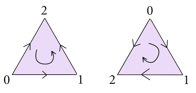
Two possible orientations of a 2-simplex
It is true, but a somewhat lengthy exercise, that the topology of a simplicial complex does not change under a consistent shuffling of the orientations across all its simplices. Nor does it change depending on how we realize a space as a simplicial complex. These kinds of results are crucial to the welfare of the theory, but have been proved once and we won’t bother reproving them here.
As a larger example, here is a simplicial complex representing the torus. It’s quite a bit more complicated than our usual quotient of a square, but it’s based on the same idea. The left and right edges are glued together, as are the top and bottom, with appropriate orientations. The only difficulty is that we need each simplex to be uniquely determined by its vertices. While this construction does not use the smallest possible number of simplices to satisfy that condition, it is the simplest to think about.
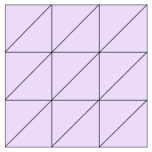
A possible realization of the torus as a simplicial complex. As an exercise, the reader is invited to fill in the orientations on the simplices to be consistent across the entire complex.
Taking a known topological space (like the torus) and realizing it as a simplicial complex is known as triangulating the space. A space which can be realized as a simplicial complex is called triangulable.
The nicest thing about the simplex is that it has an easy-to-describe boundary. Geometrically, it’s obvious: the boundary of the line segment is the two endpoints; the boundary of the triangle is the union of all three of its edges; the tetrahedron has four triangular faces as its boundary; etc. But because we need an algebraic way to describe holes, we want an algebraic way to describe the boundary. In particular, we have two important criterion that any algebraic definition must satisfy to be reasonable:
- A boundary itself has no boundary.
- The property of being boundariless (at least in low dimensions) coincides with our intuitive idea of what it means to be a loop.
Of course, just as with homotopy these holes interact in ways we’re about to see, so we need to be totally concrete before we can proceed.
The Chain Group and the Boundary Operator
In order to define an algebraic boundary, we have to realize simplices themselves as algebraic objects. This is not so difficult to do: just take all “formal sums” of simplices in the complex. More rigorously, let $ X_k$ be the set of $ k$-simplices in the simplicial complex $ X$. Define the chain group $ C_k(X)$ to be the $ \mathbb{Q}$-vector space with $ X_k$ for a basis. The elements of the $ k$-th chain group are called k-chains on $ X$. That’s right, if $ \sigma, \sigma’$ are two $ k$-simplices, then we just blindly define a bunch of new “chains” as all possible “sums” and scalar multiples of the simplices. For example, sums involving two elements would look like $ a\sigma + b\sigma’$ for some $ a,b \in \mathbb{Q}$. Indeed, we include any finite sum of such simplices, as is standard in taking the span of a set of basis vectors in linear algebra.
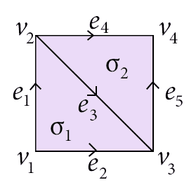
Just for a quick example, take this very simple simplicial complex:
simple-space
We’ve labeled all of the simplices above, and we can describe the chain groups quite easily. The zero-th chain group $ C_0(X)$ is the $ \mathbb{Q}$-linear span of the set of vertices $ \left \{ v_1, v_2, v_3, v_4 \right \}$. Geometrically, we might think of “the union” of two points as being, e.g., the sum $ v_1 + v_3$. And if we want to have two copies of $ v_1$ and five copies of $ v_3$, that might be thought of as $ 2v_1 + 5v_3$. Of course, there are geometrically meaningless sums like $ \frac{1}{2}v_4 – v_2 – \frac{11}{6}v_1$, but it will turn out that the algebra we use to talk about holes will not falter because of it. It’s nice to have this geometric idea of what an algebraic expression can “mean,” but in light of this nonsense it’s not a good idea to get too wedded to the interpretations.
Likewise, $ C_1(X)$ is the linear span of the set $ \left \{ e_1, e_2, e_3, e_4, e_5 \right \}$ with coefficients in $ \mathbb{Q}$. So we can talk about a “path” as a sum of simplices like $ e_1 + e_4 – e_5 + e_3$. Here we use a negative coefficient to signify that we’re travelling “against” the orientation of an edge. Note that since the order of the terms is irrelevant, the same “path” is given by, e.g. $ -e_5 + e_4 + e_1 + e_3$, which geometrically is ridiculous if we insist on reading the terms from left to right.
The same idea extends to higher dimensional groups, but as usual the visualization grows difficult. For example, in $ C_2(X)$ above, the chain group is the vector space spanned by $ \left \{ \sigma_1, \sigma_2 \right \}$. But does it make sense to have a path of triangles? Perhaps, but the geometric analogies certainly become more tenuous as dimension grows. The benefit, however, is if we come up with good algebraic definitions for the low-dimensional cases, the algebra is easy to generalize to higher dimensions.
So now we will define the boundary operator on chain groups, a linear map $ \partial : C_k(X) \to C_{k-1}(X)$ by starting in lower dimensions and generalizing. A single vertex should always be boundariless, so $ \partial v = 0$ for each vertex. Extending linearly to the entire chain group, we have $ \partial$ is identically the zero map on zero-chains. For 1-simplices we have a more substantial definition: if a simplex has its orientation as $ (v_1, v_2)$, then the boundary $ \partial (v_1, v_2)$ should be $ v_2 – v_1$. That is, it’s the front end of the edge minus the back end. This defines the boundary operator on the basis elements, and we can again extend linearly to the entire group of 1-chains.
Why is this definition more sensible than, say, $ v_1 + v_2$? Using our example above, let’s see how it operates on a “path.” If we have a sum like $ e_1 + e_4 – e_5 – e_3$, then the boundary is computed as
$ \displaystyle \partial (e_1 + e_4 – e_5 – e_3) = \partial e_1 + \partial e_4 – \partial e_5 – \partial e_3$
$$\displaystyle = (v_2 – v_1) + (v_4 – v_2) – (v_4 – v_3) – (v_3 – v_2) = v_2 – v_1$$That is, the result was the endpoint of our path $ v_2$ minus the starting point of our path $ v_1$. It is not hard to prove that this will work in general, since each successive edge in a path will cancel out the ending vertex of the edge before it and the starting vertex of the edge after it: the result is just one big alternating sum.
Even more importantly is that if the “path” is a loop (the starting and ending points are the same in our naive way to write the paths), then the boundary is zero. Indeed, any time the boundary is zero then one can rewrite the sum as a sum of “loops,” (though one might have to trivially introduce cancelling factors). And so our condition for a chain to be a “loop,” which is just one step away from being a “hole,” is if it is in the kernel of the boundary operator. We have a special name for such chains: they are called cycles.
For 2-simplices, the definition is not so much harder: if we have a simplex like $ (v_0, v_1, v_2)$, then the boundary should be $ (v_1,v_2) – (v_0,v_2) + (v_0,v_1)$. If one rewrites this in a different order, then it will become apparent that this is just a path traversing the boundary of the simplex with the appropriate orientations. We wrote it in this “backwards” way to lead into the general definition: the simplices are ordered by which vertex does not occur in the face in question ($ v_0$ omitted from the first, $ v_1$ from the second, and $ v_2$ from the third).
We are now ready to extend this definition to arbitrary simplices, but a nice-looking definition requires a bit more notation. Say we have a k-simplex which looks like $ (v_0, v_1, \dots, v_k)$. Abstractly, we can write it just using the numbers, as $ [0,1,\dots, k]$. And moreover, we can denote the removal of a vertex from this list by putting a hat over the removed index. So $ [0,1,\dots, \hat{i}, \dots, k]$ represents the simplex which has all of the vertices from 0 to $ k$ excluding the vertex $ v_i$. To represent a single-vertex simplex, we will often drop the square brackets, e.g. $ 3$ for $ [3]$. This can make for some awkward looking math, but is actually standard notation once the correct context has been established.
Now the boundary operator is defined on the standard $ n$-simplex with orientation $ [0,1,\dots, n]$ via the alternating sum
$$\displaystyle \partial([0,1,\dots, n]) = \sum_{k=0}^n (-1)^k [0, \dots, \hat{k}, \dots, n]$$It is trivial (but perhaps notationally hard to parse) to see that this coincides with our low-dimensional examples above. But now that we’ve defined it for the basis elements of a chain group, we automatically get a linear operator on the entire chain group by extending $ \partial$ linearly on chains.
Definition: The k-cycles on $ X$ are those chains in the kernel of $ \partial$. We will call k-cycles boundariless. The k-boundaries are the image of $ \partial$.
We should note that we are making a serious abuse of notation here, since technically $ \partial$ is defined on only a single chain group. What we should do is define $ \partial_k : C_k(X) \to C_{k-1}(X)$ for a fixed dimension, and always put the subscript. In practice this is only done when it is crucial to be clear which dimension is being talked about, and otherwise the dimension is always inferred from the context. If we want to compose the boundary operator in one dimension with the boundary operator in another dimension (say, $ \partial_{k-1} \partial_k$), it is usually written $ \partial^2$. This author personally supports the abolition of the subscripts for the boundary map, because subscripts are a nuisance in algebraic topology.
All of that notation discussion is so we can make the following observation: $ \partial^2 = 0$. That is, every chain which is a boundary of a higher-dimensional chain is boundariless! This should make sense in low-dimension: if we take the boundary of a 2-simplex, we get a cycle of three 1-simplices, and the boundary of this chain is zero. Indeed, we can formally prove it from the definition for general simplices (and extend linearly to achieve the result for all simplices) by writing out $ \partial^2([0,1,\dots, n])$. With a keen eye, the reader will notice that the terms cancel out and we get zero. The reason is entirely in which coefficients are negative; the second time we apply the boundary operator the power on (-1) shifts by one index. We will leave the full details as an exercise to the reader.
So this fits our two criteria: low-dimensional examples make sense, and boundariless things (cycles) represent loops.
Recasting in Algebraic Terms, and the Homology Group
For the moment let’s give boundary operators subscripts $ \partial_k : C_k(X) \to C_{k-1}(X)$. If we recast things in algebraic terms, we can call the k-cycles $ Z_k(X) = \textup{ker}(\partial_k)$, and this will be a subspace (and a subgroup) of $ C_k(X)$ since kernels are always linear subspaces. Moreover, the set $ B_k(X)$ of k-boundaries, that is, the image of $ \partial_{k+1}$, is a subspace (subgroup) of $ Z_k(X)$. As we just saw, every boundary is itself boundariless, so $ B_k(X)$ is a subset of $ Z_k(X)$, and since the image of a linear map is always a linear subspace of the range, we get that it is a subspace too.
All of this data is usually expressed in one big diagram: each of the chain groups are organized in order of decreasing dimension, and the boundary maps connect them.

chain-complex
Since our example (the “simple space” of two triangles from the previous section) only has simplices in dimensions zero, one, and two, we additionally extend the sequence of groups to an infinite sequence by adding trivial groups and zero maps, as indicated. The condition that $ \textup{im} \partial_{k+1} \subset \textup{ker} \partial_k$, which is equivalent to $ \partial^2 = 0$, is what makes this sequence a chain complex. As a side note, every sequence of abelian groups and group homomorphisms which satisfies the boundary requirement is called an algebraic chain complex. This foreshadows that there are many different types of homology theory, and they are unified by these kinds of algebraic conditions.
Now, geometrically we want to say, “The holes are all those cycles (loops) which don’t arise as the boundaries of higher-dimensional things.” In algebraic terms, this would correspond to a quotient space (really, a quotient group, which we covered in our first primer on groups) of the k-cycles by the k-boundaries. That is, a cycle would be considered a “trivial hole” if it is a boundary, and two “different” cycles would be considered the same hole if their difference is a k-boundary. This is the spirit of homology, and formally, we define the homology group (vector space) as follows.
Definition: The $ k$-th homology group of a simplicial complex $ X$, denoted $ H_k(X)$, is the quotient vector space $ Z_k(X) / B_k(X) = \textup{ker}(\partial_k) / \textup{im}(\partial_{k+1})$. Two elements of a homology group which are equivalent (their difference is a boundary) are called homologous.
The number of $ k$-dimensional holes in $ X$ is thus realized as the dimension of $ H_k(X)$ as a vector space.
The quotient mechanism really is doing all of the work for us here. Any time we have two holes and we’re wondering whether they represent truly different holes in the space (perhaps we have a closed loop of edges, and another which is slightly longer but does not quite use the same edges), we can determine this by taking their difference and seeing if it bounds a higher-dimensional chain. If it does, then the two chains are the same, and if it doesn’t then the two chains carry intrinsically different topological information.
For particular dimensions, there are some neat facts (which obviously require further proof) that make this definition more concrete.
- The dimension of $ H_0(X)$ is the number of connected components of $ X$. Therefore, computing homology generalizes the graph-theoretic methods of computing connected components.
- $ H_1(X)$ is the abelianization of the fundamental group of $ X$. Roughly speaking, $ H_1(X)$ is the closest approximation of $ \pi_1(X)$ by a $ \mathbb{Q}$ vector space.
Now that we’ve defined the homology group, let’s end this post by computing all the homology groups for this example space:
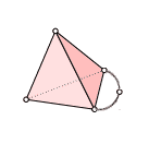
circle-wedge-sphere
This is a sphere (which can be triangulated as the boundary of a tetrahedron) with an extra “arm.” Note how the edge needs an extra vertex to maintain uniqueness. This space is a nice example because it has one-dimensional homology in dimension zero (one connected component), dimension one (the arm is like a copy of the circle), and dimension two (the hollow sphere part). Let’s verify this algebraically.
Let’s start by labelling the vertices of the tetrahedron 0, 1, 2, 3, so that the extra arm attaches at 0 and 2, and call the extra vertex on the arm 4. This completely determines the orientations for the entire simplex, as seen below.
Indeed, the chain groups are easy to write down:
$$\displaystyle C_0(X) = \textup{span} \left \{ 0,1,2,3,4 \right \}$$ $$\displaystyle C_1(X) = \textup{span} \left \{ [0,1], [0,2], [0,3], [0,4], [1,2], [1,3],[2,3],[2,4] \right \}$$ $$\displaystyle C_2(X) = \textup{span} \left \{ [0,1,2], [0,1,3], [0,2,3], [1,2,3] \right \}$$We can easily write down the images of each $ \partial_k$, they’re just the span of the images of each basis element under $ \partial_k$.
$$\displaystyle \textup{im} \partial_1 = \textup{span} \left \{ 1 – 0, 2 – 0, 3 – 0, 4 – 0, 2 – 1, 3 – 1, 3 – 2, 4 – 2 \right \}$$The zero-th homology $ H_0(X)$ is the kernel of $ \partial_0$ modulo the image of $ \partial_1$. The angle brackets are a shorthand for “span.”
$$\displaystyle \frac{\left \langle 0,1,2,3,4 \right \rangle}{\left \langle 1-0,2-0,3-0,4-0,2-1,3-1,3-2,4-2 \right \rangle}$$Since $ \partial_0$ is actually the zero map, $ Z_0(X) = C_0(X)$ and all five vertices generate the kernel. The quotient construction imposes that two vertices (two elements of the homology group) are considered equivalent if their difference is a boundary. It is easy to see that (indeed, just by the first four generators of the image) all vertices are equivalent to 0, so there is a unique generator of homology, and the vector space is isomorphic to $ \mathbb{Q}$. There is exactly one connected component. Geometrically we can realize this, because two vertices are homologous if and only if there is a “path” of edges from one vertex to the other. This chain will indeed have as its image the difference of the two vertices.
We can compute the first homology $ H_1(X)$ in an analogous way, compute the kernel and image separately, and then compute the quotient.
$$\textup{ker} \partial_1 = \textup{span} \left \{ [0,1] + [0,3] – [1,3], [0,2] + [2,3] – [0,3], [1,2] + [2,3] – [1,3], [0,1] + [1,2] – [0,2], [0,2] + [2,4] – [0,4] \right \}$$It takes a bit of combinatorial analysis to show that this is precisely the kernel of $ \partial_1$, and we will have a better method for it in the next post, but indeed this is it. As the image of $ \partial_2$ is precisely the first four basis elements, the quotient is just the one-dimensional vector space spanned by $ [0,2] + [2,4] – [0,4]$. Hence $ H_1(X) = \mathbb{Q}$, and there is one one-dimensional hole.
Since there are no 3-simplices, the homology group $ H_2(X)$ is simply the kernel of $ \partial_2$, which is not hard to see is just generated by the chain representing the “sphere” part of the space: $ [1,2,3] – [0,2,3] + [0,1,3] – [0,1,2]$. The second homology group is thus again $ \mathbb{Q}$ and there is one two-dimensional hole in $ X$.
So there we have it!
Looking Forward
Next time, we will give a more explicit algorithm for computing homology for finite simplicial complexes, and it will essentially be a variation of row-reduction which simultaneously rewrites the matrix representations of the boundary operators $ \partial_{k+1}, \partial_k$ with respect to a canonical basis. This will allow us to simply count entries on the digaonals of the two matrices, and the difference will be the dimension of the quotient space, and hence the number of holes.
Until then!