In this post we will assume the reader has a passing familiarity with some of the basic concepts of functional programming (the map, fold, and filter functions). We introduce these topics in our Racket primer, but the average reader will understand the majority of this primer without expertise in functional programming.
Follow-ups to this post can be found in the Computational Category Theory section of the Main Content page.
Preface: ML for Category Theory
A few of my readers have been asking for more posts about functional languages and algorithms written in functional languages. While I do have a personal appreciation for the Haskell programming language (and I plan to do a separate primer for it), I have wanted to explore category theory within the context of programming for quite a while now. From what I can tell, ML is a better choice than Haskell for this.
Part of the reason is that, while many Haskell enthusiasts claim it to be a direct implementation of category theory, Haskell actually tweaks category theoretic concepts in certain ways. I rest assured that the designers of Haskell (who are by assumption infinitely better at everything than I am) have very good reasons for doing this. But rather than sort through the details of the Haskell language specification to clarify the finer details, we would learn a lot more by implementing category theory by hand in a programming language that doesn’t have such concepts already.
And so we turn to ML.
ML, which stands for MetaLanguage, apparently has historical precedents for being a first in many things. One of these is an explicit recognition of parametric polymorphism, which is the idea that an operation can have the same functionality regardless of the types of the data involved; the types can, in effect, be considered variables. Another ground-breaking aspect of ML is an explicit type inference system. Similar to Haskell, an ML program will not run unless the compiler can directly prove that the program produces the correct types in every step of the computation.
Both of these features are benefits for the student of category theory. Most of our time in category theory will be spent working with very general assumptions on the capabilities of our data involved, and parametric polymorphism will be our main tool for describing what these assumptions are and for laying out function signatures.
As a side note, I’ve noticed through my ever-growing teaching experiences that one of the main things new programming students struggle with (specifically, after mastering the syntax and semantics of basic language constructs) is keeping their types straight. This is especially prominent in a language like Python (which is what I teach), where duck-typing is so convenient that it lulls the students into a false sense of security. Sooner as opposed to later they’ll add strings to numbers with the blind confidence that Python will simply get it. Around this time in their first semester of programming, I would estimate that type errors lie at the heart of 75% of the bugs my students face and fail to resolve before asking me for help. So one benefit of programming in ML for pedagogy is that it is literally impossible to make type errors. The second you try to run a program with bad types, the compiler points out what the expected type is and what the given (incorrect) type was. It takes a while to get used to type variables (and appeasing the type checker when you want to play fast and loose). But once you do you’ll find the only bugs that remain in your code are conceptual ones, which are of course much more rewarding and important bugs to fix.
So enough of this preamble. Let’s learn some ML!
Warming Up: Basic Arithmetic and Conditionals
We’ll be working with the Standard ML of New Jersey compiler, which you can download for free at their website. The file extension for ML files is .sml.
As one would expect, ML has variables and arithmetic which work in much the same way as other languages. Each variable declaration is prefixed by the word “val,” as below
val x = 7;
val y = 2;
This statements modify the global environment (the list of which variable names are associated to which values). Semicolons are required to terminate variable declarations at the global level. We can declare multiple variables in a single line using the “and” keyword
val x = 7 and y = 2;
As a precaution, “and” is only used in ML for syntactic conjunctions of variable/function declarations, and is only necessary when the two defined variable names are mutually defined in terms of each other (this can happen naturally for recursive function definitions). We will see in a moment that the logical and operation is denoted “andalso.”
We can also use pattern matching to bind these two variables in one line, much the same way as it might work in Python:
val (x,y) = (7,2);
We note that while ML does not require us to specify the type of a variable, the type is known and ever present under the surface. If we run the above code through the sml compiler (which after running the contents of a file opens a REPL to further evaluate commands), we see the following output
[opening vars.sml]
val x = 7 : int
val n = 2 : int
The environment is printed out to the user, and it displays that the two types are “int.”
Arithmetic is defined for integers, and the standard ones we will use are the expected +, -, *, and (not a slash, but) div. Here are some examples, and here is a list of all basic operations on ints. A few things to note: the unary negation operator is a tilde (~), and the semicolons are only used terminate statements in the REPL, which tells the compiler we’re ready for it to evaluate our code. Semicolons can also be used to place multiple statements on a single line of code. The “it” variable is a REPL construct which saves the most recent unbound expression evaluation.
- 3 + 6;
val it = 9 : int
- 6 div 3;
val it = 2 : int
- 2 * 9;
val it = 18 : int
- 2 - 9;
val it = ~7 : int
- ~9;
val it = ~9 : int
ML also has floating point arithmetic (in ML this type is called “real”), but treats it in a very prudish manner. Specifically (and this is a taste of the type checker doing its job too well), ML does not coerce types for you. If you want to multiply a real number and an integer, you have to first convert the int to a real and then multiply. An error will occur if you do not:
- val x = 4.0;
val x = 4.0 : real
- val y = 7;
val y = 7 : int
- x * y;
stdIn:5.1-5.6 Error: operator and operand don't agree [tycon mismatch]
  operator domain: real * real
  operand:         real * int
  in expression:
    x * y
- x * Real.fromInt(y);
val it = 28.0 : real
Here is a list of all operations on reals. We don’t anticipate using reals much, but it’s good to know that ML fervently separates them.
It seems odd that we’re talking so much about statements, because often enough we will be either binding function names (and tests) to the global environment, or restricting ourselves to local variable declarations. The latter has a slightly more complicated syntax, simply surrounding your variable declarations and evaluated code in a “let … in … end” expression. This will be a much more common construction for us.
let
   val x = 7
   val y = 9
in
   (x + 2*y) div 3
end
The “in” expression is run with the combined variables from the ambient environment (the variables declared outside of the let) and those defined inside the let. The variables defined in the let leave scope after the “in” expression is evaluated, and the entire let expression as a whole evaluates to the result of evaluating the “in” expression. Clearly and example shows what is going on much more directly than words.
The last major basic expression form are the boolean expressions and operations. The type for booleans in ML is called “bool,” and the two possible values are “true,” and “false.” They have the usual unary and binary operations, but the names are a bit weird. Binary conjunction is called “andalso,” while binary disjunction is called “orelse.”
val a = true and b = false;
val c = (a andalso b) orelse ((not a) andalso (not b));
But aside from that, boolean expressions work largely as one would expect. There are the six standard numerical comparison functions, where testing for equality is given by a single equals sign (in most languages, comparison for equality is ==), and inequality is given by the diamond operator <>. The others are, as usual, <, <=, >, >=.
- 6 = 7;
val it = false : bool
- 6 = 6;
val it = true : bool
- 6 < 7;
val it = true : bool
- 7 <= 6;
val it = false : bool
- 6 <> 7;
val it = true : bool
ML also has the standard if statement, which has the following syntax, which is more or less the same as most languages:
- val x = if 6 < 7 then ~1 else 4;
val x = ~1 : int
ML gives the programmer more or less complete freedom with whitespace, so any of these expressions can be spread out across multiple lines if the writer desires.
val x = if 6 < 7
  then
     ~1
  else
      4
This can sometimes be helpful when defining things inside of let expressions inside of function definitions (inside of other function definitions, inside of …).
So far the basics are easy, if perhaps syntactically different from most other languages we’re familiar with. So let’s move on to the true heart of ML and all functional programming languages: functions.
Functions and cases, recursion
Now that we have basic types and conditions, we can start to define some simple functions. In the global environment, functions are defined the same way as values, using the word “fun” in the place of “val.” For instance, here is a function that adds 3 to a number.
fun add3(x) = x+3
The left hand side is the function signature, and the right hand side is the body expression. As in Racket, and distinct from most imperative languages, a function evaluates to whatever the body expression evaluates to. Calling functions has two possible syntaxes:
add3(5)
add3 5
(add3 5)
In other words, if the function application is unambiguous, parentheses aren’t required. Otherwise, one can specify precedence using parentheses in either Racket (Lisp) style or in standard mathematical style.
The most significant difference between ML and most other programming languages, is that ML’s functions have case-checking. That is, we can specify what action is to be taken based on the argument, and these actions are completely disjoint in the function definition (no if statements are needed).
For instance, we could define an add3 function which nefariously does the wrong thing when the user inputs 7.
fun add3(7) = 2
  | add3(x) = x+3
The vertical bar is read “or,” and the idea is that the possible cases for the function definition must be written in most-specific to least-specific order. For example, interchanging the orders of the add3 function cases gives the following error:
- fun add3(x) = x+3
=   | add3(7) = 2;
stdIn:13.5-14.16 Error: match redundant
          x => ...
    -->   7 => ...
Functions can call themselves recursively, and this is the main way to implement loops in ML. For instance (and this is quite an inefficient example), I could define a function to check whether a number is even as follows.
fun even(0) = true
  | even(n) = not(even(n-1))
Don’t cringe too visibly; we will see recursion used in less horrifying ways in a moment.
Functions with multiple arguments are similarly easy, but there are two semantic possibilities for how to define the arguments. The first, and simplest is what we would expect from a typical language: put commas in between the arguments.
fun add(x,y) = x+y
When one calls the add function, one is forced to supply both arguments immediately. This is usually how programs are written, but often times it can be convenient to only supply one argument, and defer the second argument until later.
If this sounds like black magic, you can thank mathematicians for it. The technique is called currying, and the idea stems from the lambda calculus, in which we can model all computation using just functions (with a single argument) as objects, and function application. Numbers, arithmetic, lists, all of these things are modeled in terms of functions and function calls; the amazing thing is that everything can be done with just these two tools. If readers are interested, we could do a post or two on the lambda calculus to see exactly how these techniques work; the fun part would be that we can actually write programs to prove the theorems.
Function currying is built-in to Standard ML, and to get it requires a minor change in syntax. Here is the add function rewritten in a curried style.
fun add(x)(y) = x+y
Now we can, for instance, define the add3 function in terms of add as follows:
val add3 = add(3)
And we can curry the second argument by defining a new function which defers the first argument appropriately.
fun add6(x) = add(x)(6)
Of course, in this example addition is commutative so which argument you pick is useless.
We should also note that we can define anonymous functions as values (for instance, in a let expression) using this syntax:
val f = (fn x => x+3)
The “fn x => x+3” is just like a “lambda x: x+3” expression in Python, or a “(lambda (x) (+ x 3))” in Racket. Note that one can also define functions using the “fun” syntax in a let expression, so this is truly only for use-once function arguments.
Tuples, Lists, and Types
As we’ve discovered already, ML figures out the types of our expressions for us. That is, if we define the function “add” as above (in the REPL),
- fun add(x,y) = x+y;
val add = fn : int * int -> int
then ML is smart enough to know that “add” is to accept a list of two ints (we’ll get to what the asterisk means in a moment) and returns an int.
The curried version is similarly intuited:
- fun add(x)(y) = x+y;
val add = fn : int -> int -> int
The parentheses are implied here: int -> (int -> int). So that this is a function which accepts as input an int, and produces as output another function which accepts an int and returns an int.
But, what if we’d like to use “add” to add real numbers? ML simply won’t allow us to; it will complain that we’re providing the wrong types. In order to make things work, we can tell ML that the arguments are reals, and it will deduce that “+” here means addition on reals and not addition on ints. This is one awkward thing about ML; while the compiler is usually able to determine the most general possible type for our functions, it has no general type for elements of a field, and instead defaults to int whenever it encounters arithmetic operations. In any case, this is how to force a function to have a type signature involving reals:
- fun add(x:real, y:real) = x+y;
val add = fn : real * real -> real
If we’re going to talk about types, we need to know all of ML’s syntax for its types. Of course there are the basics (int, real, bool). Then there are function types: int -> int is the type of a function which accepts one int and returns an int.
We’ll see two new types in this section, and the first is the tuple. In ML, tuples are heterogeneous, so we can mix types in them. For instance,
- val tup = (true, 7, 4.4);
val tup = (true,7,4.4) : bool * int * real
Here the asterisk denotes the tuple type, and one familiar with set theory can think of a tuple as an element of the product of sets, in this case
$$\displaystyle \left \{ \textup{true}, \textup{false} \right \} \times \mathbb{Z} \times \mathbb{R}$$Indeed, there is a distinct type for each possible kind of tuple. A tuple of three ints (int * int * int) is a distint type from a tuple of three booleans (bool * bool * bool). When we define a function that has multiple arguments using the comma syntax, we are really defining a function which accepts as input a single argument which is a tuple. This parallels exactly how functions on multiple arguments work in classical mathematics.
The second kind of compound type we’ll use quite often is the list. Lists are distinct from tuples in ML in that lists must be homogenous. So a list of integers (which has type “int list”) is different from a list of booleans.
The operations on lists are almost identical as in Haskell. To construct explicit lists use square brackets with comma-delimited elements. To construct them one piece at a time, use the :: list constructor operation. For those readers who haven’t had much experience with lists in functional programming: all lists are linked lists, and the :: operation is the operation of appending a single value to the beginning of a given list. Here are some examples.
- val L = [1,2,3];
val L = [1,2,3] : int list

- val L = 1::(2::(3::nil));
val L = [1,2,3] : int list
The “nil” expression is the empty list, as is the empty-square-brackets expression “[]”.
There is a third kind of compound type called the record, and it is analogous to a C struct, where each field is named. We will mention this in the future once we have a need for it.
The most important thing about lists and tuples in ML is that functions which operate on them don’t always have an obvious type signature. For instance, here is a function which takes in a tuple of two elements and returns the first element.
fun first(x,y) = x
What should the type of this function be? We want it to be able to work with any tuple, no matter the type. As it turns out, ML was one of the first programming language to allow this sort of construction to work. The formal name is parametric polymorphism. It means that a function can operate on many different kinds of types (because the actual computation is the same regardless of the types involved) and the full type signature can be deduced for each function call based on the parameters for that particular call.
The other kind of polymorphism is called ad-hoc polymorphism. Essentially this means that multiple (very different) operations can have the same name. For instance, addition of integers and addition of floating point numbers require two very different sets of instructions, but they both go under the name of +.
What ML does to make its type system understand parametric polymorphism is introduce so-called type variables. A type variable is any string prefixed by a single quote, e.g. ‘a, and they can represent any type. When ML encounters a function with an ambiguous type signature, it decides what the most general possible type is (which usually involves a lot of type variables), and then uses that type.
So to complete our example, the first function has the type
'a * 'b -> 'a
As a side note, the “first” function is in a sense the “canonical” operation that has this type signature. If nothing is known about the types, then no other action can happen besides the projection. There are some more interesting things to be said about such canonical operations (for instance, could we get away with not having to even define them at all).
The analogous version for lists is as follows. Note that in order to decompose a list into its first element and the tail list, we need to use pattern matching.
fun listFirst([x]) = x
  | listFirst(head::tail) = head
And this function has the type signature ‘a list -> ‘a. As a slightly more complicated example (where we need recursion), we can write a function to test for list membership.
fun member(x, nil) = false
  | member(x, (head::tail)) = if x = head then true
                              else member(x, tail)
If you run this program and see some interesting warning messages, see this StackOverflow question for a clarification.
Defining New Types
The simplest way to define a new type is to just enumerate all possibilities. For instance, here is an enumerated datatype with four possibilities.
datatype maths = algebra | analysis | logic | computation
Then we can define functions which operate on those types using pattern matching.
fun awesome(algebra) = true
  | awesome(analysis) = false
  | awesome(logic) = false
  | awesome(computation) = true
And this function has type maths -> bool (don’t take it too seriously :-)). We can also define data types whose constructors require arguments.
datatype language = functional of string*bool
                  | imperative of string
                  | other
Here we define a language to be functional or imperative. The functional type consists of a name and a boolean representing whether it is purely functional, while the imperative type just consists of a name. We can then construct these types by treating the type constructors as if they were functions.
val haskell = functional("Haskell", true) and
    java = imperative("Java") and
    prolog = other;
Perhaps more useful than this is to define types using type variables. A running example we will use for the remainder of this post is a binary tree of homogeneous elements at each node. Defining such types is easy: all one needs to do is place the appropriate type (with parentheses to clarify when the description of a type starts or ends) after the “of” keyword.
datatype 'a Tree = empty
                 | leaf of 'a
                 | node of (('a Tree) * 'a * ('a Tree))
We can create instances of an integer tree as expected:
val t2 = node(node(leaf(2), 3, leaf(4)), 6, leaf(8))
The TreeSort Algorithm
We can define a host of useful operations on trees (of any type). For instance, below we compute the breadth of a tree (the total number of leaves), the depth of a tree (the maximal length of a path from the root to a leaf), and the ability to flatten a tree (traverse the tree in order and place all of the values into a list). These first two are a nice warm-up.
fun breadth(empty) = 0
  | breadth(leaf(_)) = 1
  | breadth(node(left, _, right)) = breadth(left) + breadth(right)
Here the underscore indicates a pattern match with a variable we won’t actually use. This is more space efficient for the compiler; it can avoid adding extra values to the current environment in a potentially deep recursion.
fun depth(empty) = 0
  | depth(leaf(_)) = 1
  | depth(node(left, _, right)) =
      let
         val (lDepth, rDepth) = (1 + depth(left), 1 + depth(right))
      in
         if lDepth > rDepth then lDepth else rDepth
      end
This function should be self explanatory.
fun flatten(empty) = []
   | flatten(leaf(x)) = [x]
   | flatten(node(left, x, right)) =
               flatten(left) @ (x :: flatten(right))
Here the @ symbol is list concatenation. This is not quite the most efficient way to do this (we are going to write a forthcoming post about tail-call optimization, and there we will see why), but it is certainly the clearest. In the final recursive call, we traverse the left subtree first, flattening it into a list in order. Then we flatten the right hand side, and put the current node’s element in between the two flattened parts.
Note that if our tree is ordered, then flatten will produce a strictly increasing list of the elements in the tree. For those readers unfamiliar with ordered binary trees, for all intents and purposes this is an “int Tree” and we can compare the values at different nodes. Then an ordered binary tree is a tree which satisfies the following property for each node: all of the values in the left child’s subtree are strictly smaller than the current node’s value, and all of the values in the right child’s subtree are greater than or equal to the current node’s value.
Indeed, we can use the flatten function as part of a simple algorithm to sort lists of numbers. First we insert the numbers in the unsorted list into a tree (in a way that preserves the ordered property at each step), and then we flatten the tree into a sorted list. This algorithm is called TreeSort, and the insert function is simple as well.
fun insert(x, empty) = leaf(x)
  | insert(y, leaf(x)) = if x <= y
                         then node(empty, x, leaf(y))
                         else node(leaf(y), x, empty)
  | insert(y, node(left, x, right)) =
                if x <= y
                then node(left, x, insert(y, right))
                else node(insert(y, left), x, right)
If we’re at a nonempty node, then we just recursively insert into the appropriate subtree (taking care to create new interior nodes if we’re at a leaf). Note that we do not do any additional computation to ensure that the tree is balanced (that each node has approximately as many children in its left subtree as in its right). Doing so would digress from the point of this primer, but rest assured that the problem of keeping trees balanced has long been solved.
Now the process of calling insert on every element of a list is just a simple application of fold. ML does have the standard map, foldl, foldr, and filter functions, although apparently filter is not available in the standard library (one needs to reference the List module via List.filter).
In any case, foldl is written in the currying style and building the tree is a simple application of it. As we said, the full sorting algorithm is just the result of flattening the resulting tree with our in-order traversal.
fun sort(L) = flatten(foldl(insert)(empty)(L))
So there you have it! One of the simplest (efficient) sorting algorithms I can think of in about twelve lines of code.
Free Monoid Homomorphisms: A More Advanced Example
Just to get a quick taste of what our series on category theory will entail, let’s write a program with a slightly more complicated type signature. The idea hinges on the idea that lists form a what’s called a free monoid. In particular,
Definition: A monoid is a set $ X$ equipped with an associative binary operation $ \cdot: X \times X \to X$ and an identity element $ 1 \in X$ for which $ x1 = 1x = x$ for all $ x \in X$.
Those readers who have been following our series on group theory will recognize a monoid as a group with less structure (there is no guarantee of inverses for the $ \cdot$ operation). The salient fact for this example is that the set of ML values of type $ \textup{‘a list}$ forms a monoid. The operation is list concatenation, and the identity element is the empty list. Call the empty list nil and the append operation @, as it is in ML.
More than that, $ \textup{‘a list}$ forms a free monoid, and the idea of freeness has multiple ways of realization. One sort of elementary way to understand freeness is that the only way to use the binary operation to get to the identity is to have the two summands both be the identity element. In terms of lists, the only way to concatenate two lists to get the empty list is to have both pieces be empty to begin with.
Another, more mature (more category-theoretical) way to think about freeness is to say is satisfies the following “universal” property. Call $ A$ the set of values of type ‘a, and $ [A]$ the set of values of type $ \textup{‘a list}$, and suppose that $ (B, \cdot_B, 1_B)$ is the datum of an arbitrary monoid. The universal property says that if we are given a function $ f: A \to B$, and we take the canonical map $ g: A \to [A]$ which maps an element $ a \in A$ to the single-entry list $ [a] \in [A]$, then there is a unique way to extend $ f$ to a monoid homomorphism $ f^* : [A] \to B$ on lists, so that $ f^*g = f$. We have mentioned monoid homomorphisms on this blog before in the context of string metrics, but briefly a monoid homomorphism respects the monoid structure in the sense that (for this example) $ f^*(a \textup{ @ } b) = f^*(a) \cdot_B f^*(b)$ no matter what $ a, b$ are.
This was quite a mouthful, but the data is often written in terms of a so-called “commutative diagram,” whose general definition we will defer to a future post. The diagram for this example looks like:
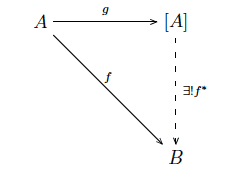
monoid-hom-freeness
The dashed line says we are asserting the existence of $ f^*$, and the symbol $ \exists !$ says this function exists and is uniquely determined by $ f, g$. The diagram “commutes” in the sense that traveling from $ A$ to $ B$ along $ f$ gives you the same computational result as traveling by $ g$ and then $ f^*$. The reason for the word “universal” will become clear in future posts, but vaguely it’s because the set $ [A]$ is a unique “starting place” in a special category.
If this talk is too mysterious, we can just go ahead and prove that $ f^*$ exists by writing a program that computes the function transforming $ f \mapsto f^*$. We call the function “listMonoidLift” because it “lifts” the function $ f$ from just operating on $ A$ to the status of a monoid homomorphism. Very regal, indeed.
Part of the beauty of this function is that a number of different list operations (list length, list sum, member tests, map, etc.), when viewed under this lens, all become special cases of this theorem! By thinking about things in terms of monoids, we write less code, and more importantly we recognize that these functions all have the same structural signature. Perhaps one can think of it like parametric polymorphism on steroids.
fun listMonoidLift(f:('a->'b), (combine:(('b * 'b) -> 'b), id:'b)) =
   let
      fun f'(nil) = id
        | f'(head::tail) = combine(f(head), f'(tail))
   in
      f'
   end
Here we specified the types of the input arguments to be completely clear what’s what. The first argument is our function $ f$ as in the above diagram, and the second two arguments together form the data of our monoid (the set $ B$ is implicitly the collection of types $ ‘b$ determined at the time of the function call). Now let’s see how the list summation and list length functions can be written in terms of the listMonoidLift function.
fun plus(x, y) = x + y
val sum = listMonoidLift((fn x => x), (plus, 0))
val length = listMonoidLift((fn x => 1), (plus, 0))
The plus function on integers with zero as the identity is the monoid $ B$ in both cases (and also happens to be $ A$ by coincidence), but in the summation case the function $ f$ is the identity and for length it is the constant $ 1$ function.
As a more interesting example, see how list membership is a lift.
fun member(x) = listMonoidLift((fn y => y = x),
                      ((fn (a,b) => a orelse b), false))
Here the member function is curried; it has type ‘a -> ‘a list -> bool (though it’s a bit convoluted since listMonoidLift is what’s returning the ‘a list -> bool part of the type signature). Here the $ B$ monoid is the monoid of boolean values, where the operation is logical “or” and the identity is false. It is a coincidence and a simple exercise to prove that $ B$ is a free monoid as well.
Now the mapping $ f(y)$ is the test to see if $ y$ is the same object as $ x$. The lift to the list monoid will compute the logical “or” of all evaluations of $ f$ on the values.
Indeed, (although this author hates bringing up too many buzzwords where they aren’t entirely welcome) the monoid lifting operation we’ve just described is closely related to the MapReduce framework (without all the distributed computing parts). Part of the benefit of MapReduce is that the programmer need only define the Map() and Reduce() functions (the heart of the computation) and MapReduce does the rest. What this example shows is that defining the Map() function can be even simpler: one only needs define the function $ f$, and Map() is computed as $ f^*$ automatically. The Reduce() part is simply the definition of the target monoid $ B$.
Just to drive this point home, we give the reader a special exercise: write map as a special case of listMonoidLift. The result (the map function) should have one of the two type signatures:
map : ('a -> 'b) * ('a list) -> 'b list
map : 'a -> 'b -> 'a list -> b' list
As a hint, the target monoid should also be a list monoid.
Part of why this author is hesitant to bring up contemporary software in discussing these ideas is because the ideas themselves are far from contemporary. Burstall and Landin’s, 1969 text Programs and Their Proofs (which this author would love to find a copy of) details this exact reduction and other versions of this idea in a more specific kind of structure called “free algebras.” So MapReduce (minus the computer programs and distributed systems) was a well-thought-out idea long before the internet or massively distributed systems were commonplace.
In any case, we’ll start the next post in this series right off with the mathematical concept of a category. We’ll start slow and detail many examples of categories that show up both in (elementary) mathematics and computing, and then move on to universal properties, functors, natural transformations, and more, implementing the ideas all along the way.
Until then!
Want to respond? Send me an email, post a webmention, or find me elsewhere on the internet.