Previously on this blog, we’ve covered two major kinds of algebraic objects: the vector space and the group. There are at least two more fundamental algebraic objects every mathematician should something know about. The first, and the focus of this primer, is the ring. The second, which we’ve mentioned briefly in passing on this blog, is the field. There are a few others important to the pure mathematician, such as the $ R$-module (here $ R$ is a ring). These do have some nice computational properties, but in order to even begin to talk about them we need to know about rings.
A Very Special Kind of Group
Recall that an abelian group $ (G, +)$ is a set $ G$ paired with a commutative binary operation $ +$, where $ G$ has a special identity element called 0 which acts as an identity for $ +$. The archetypal example of an abelian group is, of course, the integers $ \mathbb{Z}$ under addition, with zero playing the role of the identity element.
The easiest way to think of a ring is as an abelian group with more structure. This structure comes in the form of a multiplication operation which is “compatible” with the addition coming from the group structure.
Definition: A ring $ (R, +, \cdot)$ is a set $ R$ which forms an abelian group under $ +$ (with additive identity 0), and has an additional associative binary operation $ \cdot$ with an element 1 serving as a (two-sided) multiplicative identity. Furthermore, $ \cdot$ distributes over $ +$ in the sense that for all $ x,y,z \in R$
$$x(y+z) = xy + xz$ and $ (y+z)x = yx + zx$$The most important thing to note is that multiplication is not commutative both in general rings and for most rings in practice. If multiplication is commutative, then the ring is called commutative. Some easy examples of commutative rings include rings of numbers like $ \mathbb{Z}, \mathbb{Z}/n\mathbb{Z}, \mathbb{Q}, \mathbb{R}$, which are just the abelian groups we know and love with multiplication added on.
If the reader takes anything away from this post, it should be the following:
Rings generalize arithmetic with integers.
Of course, this would imply that all rings are commutative, but this is not the case. More meaty and tempestuous examples of rings are very visibly noncommutative. One of the most important examples are rings of matrices. In particular, denote by $ M_n(\mathbb{R})$ the set of all $ n \times n$ matrices with real valued entries. This forms a ring under addition and multiplication of matrices, and has as a multiplicative identity the $ n \times n$ identity matrix $ I_n$.
Commutative rings are much more well-understood than noncommutative rings, and the study of the former is called commutative algebra. This is the main prerequisite for fields like algebraic geometry, which (in the simplest examples) associate commutative rings to geometric objects.
For us, all rings will have an identity, but many ring theorists will point out that one can just as easily define a ring to not have a multiplicative identity. We will call these non-unital rings, and will rarely, if ever, see them on this blog.
Another very important example of a concrete ring is the polynomial ring in $ n$ variables with coefficients in $ \mathbb{Q}$ or $ \mathbb{R}$. This ring is denoted with square brackets denoting the variables, e.g. $ \mathbb{R}[x_1, x_2, \dots , x_n]$. We rest assured that the reader is familiar with addition and multiplication of polynomials, and that this indeed forms a ring.
Kindergarten Math
Let’s start with some easy properties of rings. We will denote our generic ring by $ R$.
First, the multiplicative identity of a ring is unique. The proof is exactly the same as it was for groups, but note that identities must be two-sided for this to work. If $ 1, 1’$ are two identities, then $ 1 = 1 \cdot 1′ = 1’$.
Next, we prove that $ 0a = a0 = 0$ for all $ a \in R$. Indeed, by the fact that multiplication distributes across addition, $ 0a = (0 + 0)a = 0a + 0a$, and additively canceling $ 0a$ from both sides gives $ 0a = 0$. An identical proof works for $ a0$.
In fact, pretty much any “obvious property” from elementary arithmetic is satisfied for rings. For instance, $ -(-a) = a$ and $ (-a)b = a(-b) = -(ab)$ and $ (-1)^2 = 1$ are all trivial to prove. Here is a list of these and more properties which we invite the reader to prove.
Zero Divisors, Integral Domains, and Units
One thing that is very much not automatically given in the general theory of rings is multiplicative cancellation. That is, if I have $ ac = bc$ then it is not guaranteed to be the case that $ a = b$. It is quite easy to come up with examples in modular arithmetic on integers; if $ R = \mathbb{Z}/8\mathbb{Z}$ then $ 2*6 = 6*6 = 4 \mod 8$, but $ 2 \neq 6$.
The reason for this phenomenon is that many rings have elements that lack multiplicative inverses. In $ \mathbb{Z}/8\mathbb{Z}$, for instance, $ 2$ has no multiplicative inverse (and neither does 6). Indeed, one is often interested in determining which elements are invertible in a ring and which elements are not. In a seemingly unrelated issue, one is interested in determining whether one can multiply any given element $ x \in R$ by some $ y$ to get zero. It turns out that these two conditions are disjoint, and closely related to our further inspection of special classes of rings.
Definition: An element $ x$ of a ring $ R$ is said to be a left zero-divisor if there is some $ y \neq 0$ such that $ xy = 0$. Similarly, $ x$ is a right zero-divisor if there is a $ z$ for which $ zx = 0$. If $ x$ is a left and right zero-divisor (e.g. if $ R$ is commutative), it is just called a zero-divisor.
Definition: Let $ x,y \in R$. The element $ y$ is said to be a left inverse to $ x$ if $ yx = 1$, and a right inverse if $ xy = 1$. If there is some $ z \neq 0$ for which $ xz = zx = 1$, then $ x$ is said to be a two-sided inverse and $ z$ is called the inverse of $ x$, and $ x$ is called a unit.
As a quick warmup, we prove that if $ x$ has a left and a right inverse then it has a two-sided inverse. Indeed, if $ zx = 1 = xy$, then $ z = z(xy) = (zx)y = y$, so in fact the left and right inverses are the same.
The salient fact here is that having a (left- or right-) inverse allows one to do (left- or right-) cancellation, since obviously when $ ac = bc$ and $ c$ has a right inverse, we can multiply $ acc^{-1} = bcc^{-1}$ to get $ a=b$. We will usually work with two-sided inverses and zero-divisors (since we will usually work in a commutative ring). But in non-commutative rings, like rings of matrices, one-sided phenomena do run rampant, and one must distinguish between them.
The right way to relate these two concepts is as follows. If $ c$ has a right inverse, then define the right-multiplication function $ (- \cdot c) : R \to R$ which takes $ x$ and spits out $ xc$. In fact, this function is an injection. Indeed, we already proved that (because $ c$ has a right inverse) if $ xc = yc$ then $ x = y$. In particular, there is a unique preimage of $ 0$ under this map. Since $ 0c = 0$ is always true, then it must be the case that the only way to left-multiply $ c$ times something to get zero is $ 0c$. That is, $ c$ is not a right zero-divisor if right-multiplication by $ c$ is injective. On the other hand, if the map is not injective, then there are some $ x \neq y$ such that $ xc = yc$, implying $ (x-y)c = 0$, and this proves that $ c$ is a right zero-divisor. We can do exactly the same argument with left-multiplication.
But there is one minor complication: what if right-multiplication is injective, but $ c$ has no inverses? It’s not hard to come up with an example: 2 as an element of the ring of integers $ \mathbb{Z}$ is a perfectly good one. It’s neither a zero-divisor nor a unit.
This basic study of zero-divisors gives us some natural definitions:
Definition: A division ring is a ring in which every element has a two-sided inverse.
If we allow that $ R$ is commutative, we get something even better (more familiar: $ \mathbb{Q}, \mathbb{R}, \mathbb{C}$ are the standard examples of fields).
Definition: A field is a nonzero commutative division ring.
The “nonzero” part here is just to avoid the case when the ring is the trivial ring (sometimes called the zero ring) with one element. i.e., the set $ \left \{ 0 \right \}$ is a ring in which zero satisfies both the additive and multiplicative identities. The zero ring is excluded from being a field for silly reasons: elegant theorems will hold for all fields except the zero ring, and it would be messy to require every theorem to add the condition that the field in question is nonzero.
We will have much more to say about fields later on this blog, but for now let’s just state one very non-obvious and interesting result in non-commutative algebra, known as Wedderburn’s Little Theorem.
Theorem: Every finite divison ring is a field.
That is, simply having finitely many elements in a division ring is enough to prove that multiplication is commutative. Pretty neat stuff. We will actually see a simpler version of this theorem in a moment.
Now as we saw units and zero-divisors are disjoint, but not quite opposites of each other. Since we have defined a division ring as a ring where all (non-zero) elements are units, it is natural to define a ring in which the only zero-divisor is zero. This is considered a natural generalization of our favorite ring $ \mathbb{Z}$, hence the name “integral.”
Definition: An integral domain is a commutative ring in which zero is the only zero-divisor.
Note the requirement that the ring is commutative. Often we will simply call it a domain, although most authors allow domains to be noncommutative.
Already we can prove a very nice theorem:
Theorem: Every finite integral domain is a field.
Proof. Integral domains are commutative by definition, and so it suffices to show that every non-zero element has an inverse. Let $ R$ be our integral domain in question, and $ x \in R$ the element whose inverse we seek. By our discussion of above, right multiplication by $ x$ is an injective map $ R \to R$, and since $ R$ is finite this map must be a bijection. Hence $ x$ must have some $ y \neq 0$ so that $ yx = 1$. And so $ y$ is the inverse of $ x$.
$$\square$$We could continue traveling down this road of studying special kinds of rings and their related properties, but we won’t often use these ideas on this blog. We do think the reader should be familiar with the names of these special classes of rings, and we will state the main theorems relating them.
Definition: A nonzero element $ p \in R$ is called prime if whenever $ p$ divides a product $ ab$ it either divides $ a$ or $ b$ (or both). A unique factorization domain (abbreviated UFD) is an integral domain in which every element can be written uniquely as a product of primes.
Definition: A Euclidean domain is a ring in which the division algorithm can be performed. That is, there is a norm function $ | \cdot | : R \\ \left \{ 0 \right \} \to \mathbb{N}$, for which every pair $ a,b \neq 0$ can be written as $ a = bq + r$ with r satisfying $ |r| < |b|$.
Paolo Aluffi has a wonderful diagram showing the relations among the various special classes of integral domains. This image comes from his book, Algebra: Chapter 0, which is a must-have for the enterprising mathematics student interested in algebra.
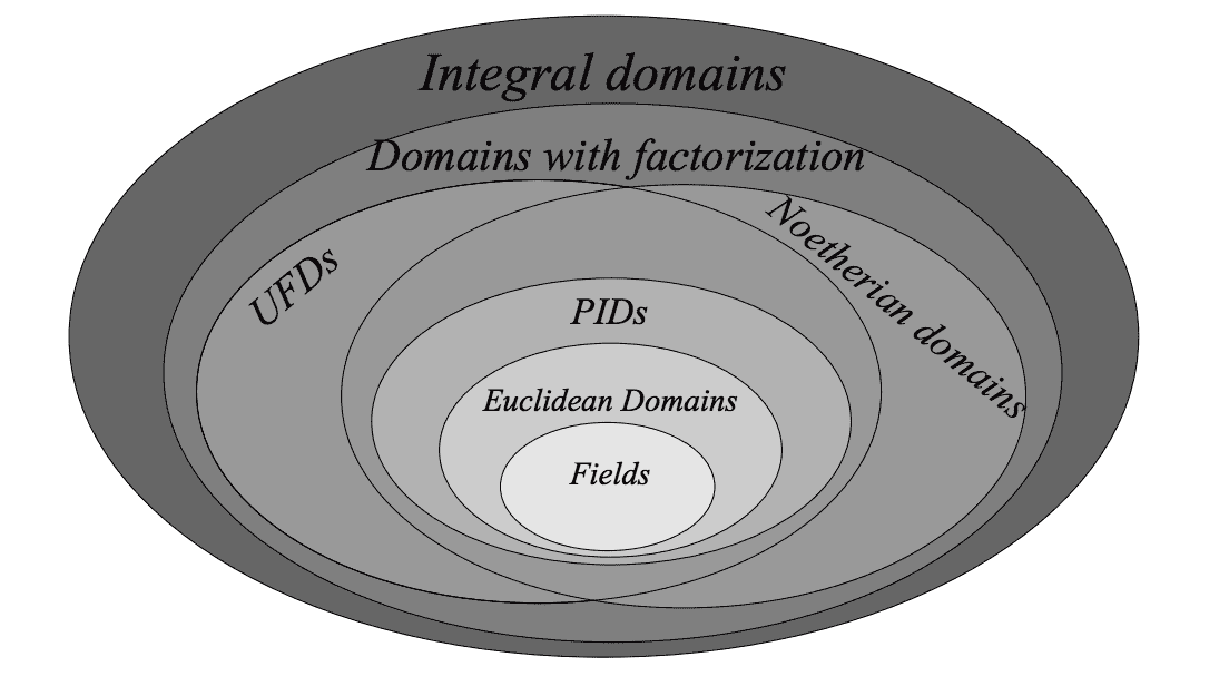
rings
In terms of what we have already seen, this diagram says that every field is a Euclidean domain, and in turn every Euclidean domain is a unique factorization domain. These are standard, but non-trivial theorems. We will not prove them here.
The two big areas in this diagram we haven’t yet mentioned on this blog are PIDs and Noetherian domains. The reason for that is because they both require a theory of ideals in rings (perhaps most briefly described as a generalization of the even numbers). We will begin next time with a discussion of ideals, and their important properties in studying rings, but before we finish we want to focus on one main example that will show up later on this blog.
Polynomial Rings
Let us formally define the polynomial ring.
Definition: Let $ R$ be a commutative ring. Define the ring $ R[x]$, to be the set of all polynomials in $ x$ with coefficients in $ R$, where addition and multiplication are the usual addition and multiplication of polynomials. We will often call $ R[x]$ the polynomial ring in one variable over $ R$.
We will often replace $ x$ by some other letter representing an “indeterminate” variable, such as $ t$, or $ y$, or multiple indexed variables as in the following definition.
Definition: Let $ R$ be a commutative ring. The ring $ R[x_1, x_2, \dots, x_n]$ is the set of all polynomials in the $ n$ variables with the usual addition and multiplication of polynomials.
What can we say about the polynomial ring in one variable $ R[x]$? It’s additive and multiplicative identities are clear: the constant 0 and 1 polynomials, respectively. Other than that, we can’t quite get much more. There are some very bizarre features of polynomial rings with bizarre coefficient rings, such as multiplication decreasing degree.
However, when we impose additional conditions on $ R$, the situation becomes much nicer.
Theorem: If $ R$ is a unique factorization domain, then so is $ R[x]$.
Proof. As we have yet to discuss ideals, we refer the reader to this proof, and recommend the reader return to it after our next primer.
$$\square$$On the other hand, we will most often be working with polynomial rings over a field. And here the situation is even better:
Theorem: If $ k$ is a field, then $ k[x]$ is a Euclidean domain.
Proof. The norm function here is precisely the degree of the polynomial (the highest power of a monomial in the polynomial). Then given $ f,g$, the usual algorithm for polynomial division gives a quotient and a remainder $ q, r$ so that $ f = qg + r$. In following the steps of the algorithm, one will note that all multiplication and division operations are performed in the field $ k$, and the remainder always has a smaller degree than the quotient. Indeed, one can explicitly describe the algorithm and prove its correctness, and we will do so in full generality in the future of this blog when we discuss computational algebraic geometry.
$$\square$$For multiple variables, things are a bit murkier. For instance, it is not even the case that $ k[x,y]$ is a euclidean domain. One of the strongest things we can say originates from this simple observation:
Lemma: $ R[x,y]$ is isomorphic to $ R[x][y]$.
We haven’t quite yet talked about isomorphisms of rings (we will next time), but the idea is clear: every polynomial in two variables $ x,y$ can be thought of as a polynomial in $ y$ where the coefficients are polynomials in $ x$ (gathered together by factoring out common factors of $ y^k$). Similarly, $ R[x_1, \dots, x_n]$ is the same thing as $ R[x_1, \dots, x_{n-1}][x_n]$ by induction. This allows us to prove that any polynomial ring is a unique factorization domain:
Theorem: If $ R$ is a UFD, so is $ R[x_1, \dots, x_n]$.
Proof. $ R[x]$ is a UFD as described above. By the lemma, $ R[x_1, \dots, x_n] = R[x_1, \dots, x_{n-1}][x_n]$ so by induction $ R[x_1, \dots, x_{n-1}]$ is a UFD implies $ R[x_1, \dots, x_n]$ is as well.
$$\square$$We’ll be very interested in exactly how to compute useful factorizations of polynomials into primes when we start our series on computational algebraic geometry. Some of the applications include robot motion planning, and automated theorem proving.
Next time we’ll visit the concept of an ideal, see quotient rings, and work toward proving Hilbert’s Nullstellensatz, a fundamental result in algebraic geometry.
Until then!
Want to respond? Send me an email, post a webmention, or find me elsewhere on the internet.