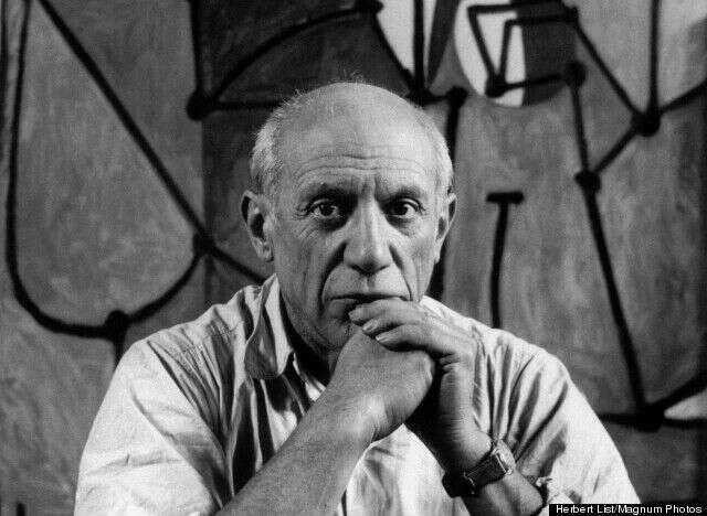
Pablo Picasso
Simplicity and the Artist
Some of my favorite of Pablo Picasso’s works are his line drawings. He did a number of them about animals: an owl, a camel, a butterfly, etc. This piece called “Dog” is on my wall:
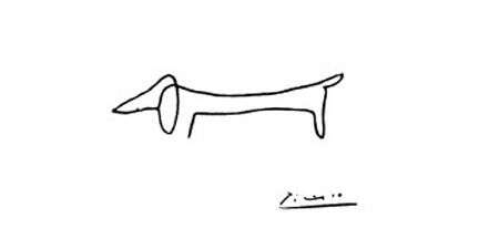
Dachshund-Picasso-Sketch
(Jump to interactive demo where we recreate “Dog” using the math in this post)
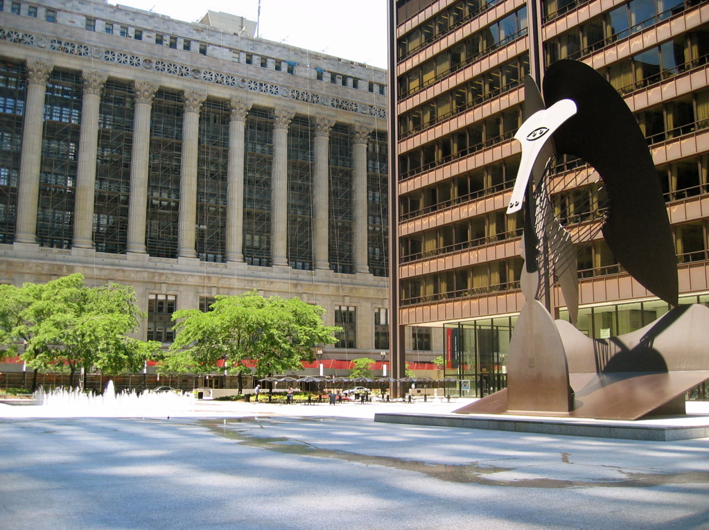
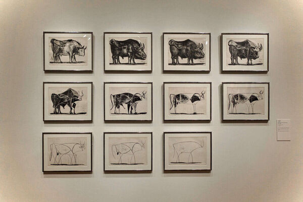
These paintings are extremely simple but somehow strike the viewer as deeply profound. They give the impression of being quite simple to design and draw. A single stroke of the hand and a scribbled signature, but what a masterpiece! It simultaneously feels like a hasty afterthought and a carefully tuned overture to a symphony of elegance. In fact, we know that Picasso’s process was deep. For example, in 1945-1946, Picasso made a series of eleven drawings (lithographs, actually) showing the progression of his rendition of a bull. The first few are more or less lifelike, but as the series progresses we see the bull boiled down to its essence, the final painting requiring a mere ten lines. Along the way we see drawings of a bull that resemble some of Picasso’s other works (number 9 reminding me of the sculpture at Daley Center Plaza in Chicago). Read more about the series of lithographs here.
the bull
Now I don’t pretend to be a qualified artist (I couldn’t draw a bull to save my life), but I can recognize the mathematical aspects of his paintings, and I can write a damn fine program. There is one obvious way to consider Picasso-style line drawings as a mathematical object, and it is essentially the Bezier curve. Let’s study the theory behind Bezier curves, and then write a program to draw them. The mathematics involved requires no background knowledge beyond basic algebra with polynomials, and we’ll do our best to keep the discussion low-tech. Then we’ll explore a very simple algorithm for drawing Bezier curves, implement it in Javascript, and recreate one of Picasso’s line drawings as a sequence of Bezier curves.
The Bezier Curve and Parameterizations
When asked to conjure a “curve” most people (perhaps plagued by their elementary mathematics education) will either convulse in fear or draw part of the graph of a polynomial. While these are fine and dandy curves, they only represent a small fraction of the world of curves. We are particularly interested in curves which are not part of the graphs of any functions.
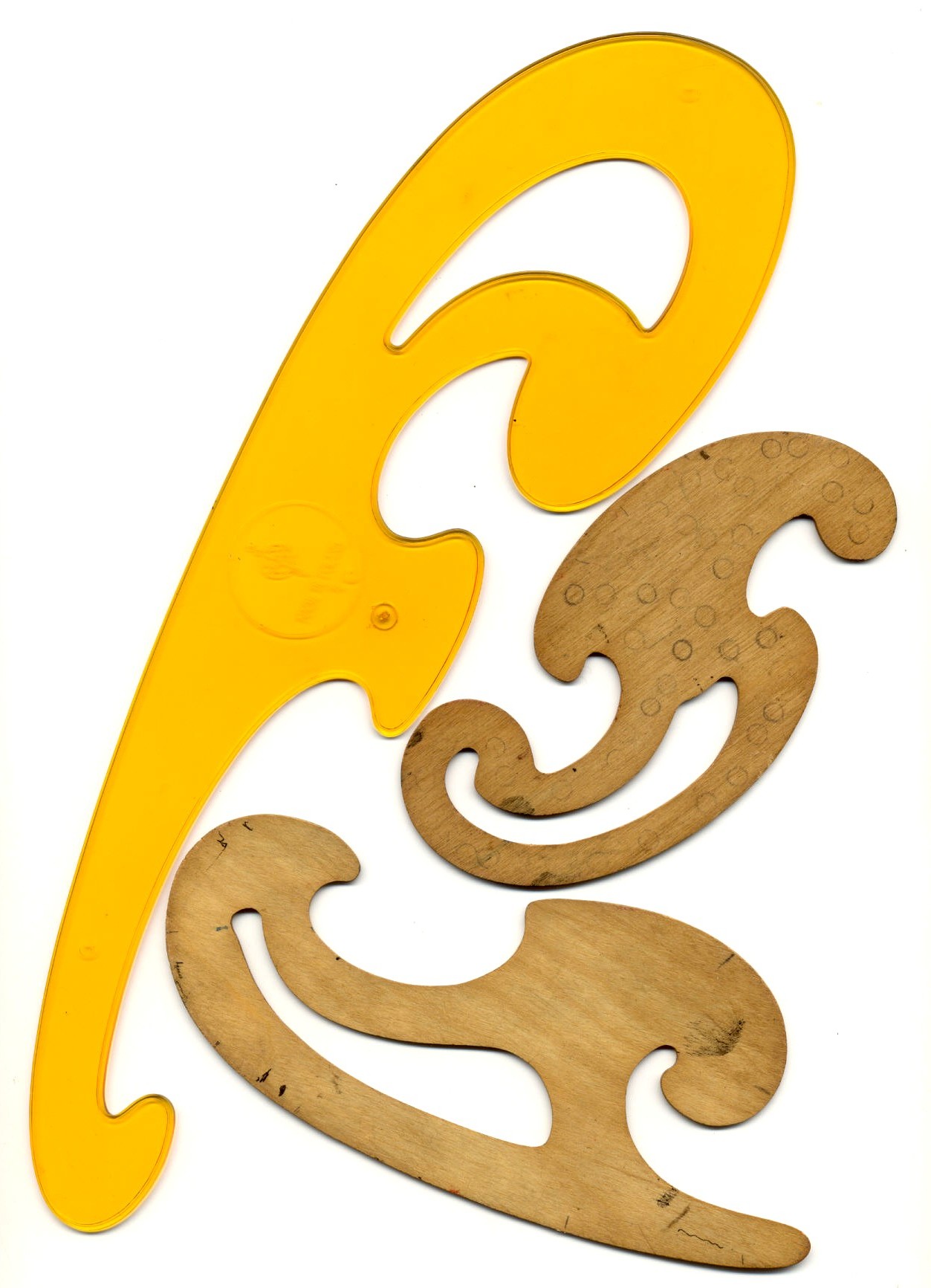
For instance, a French curve is a physical template used in (manual) sketching to aid the hand in drawing smooth curves. Tracing the edges of any part of these curves will usually give you something that is not the graph of a function. It’s obvious that we need to generalize our idea of what a curve is a bit. The problem is that many fields of mathematics define a curve to mean different things. The curves we’ll be looking at, called Bezier curves, are a special case of single-parameter polynomial plane curves. This sounds like a mouthful, but what it means is that the entire curve can be evaluated with two polynomials: one for the $ x$ values and one for the $ y$ values. Both polynomials share the same variable, which we’ll call $ t$, and $ t$ is evaluated at real numbers.
An example should make this clear. Let’s pick two simple polynomials in $ t$, say $ x(t) = t^2$ and $ y(t) = t^3$. If we want to find points on this curve, we can just choose values of $ t$ and plug them into both equations. For instance, plugging in $ t = 2$ gives the point $ (4, 8)$ on our curve. Plotting all such values gives a curve that is definitely not the graph of a function:
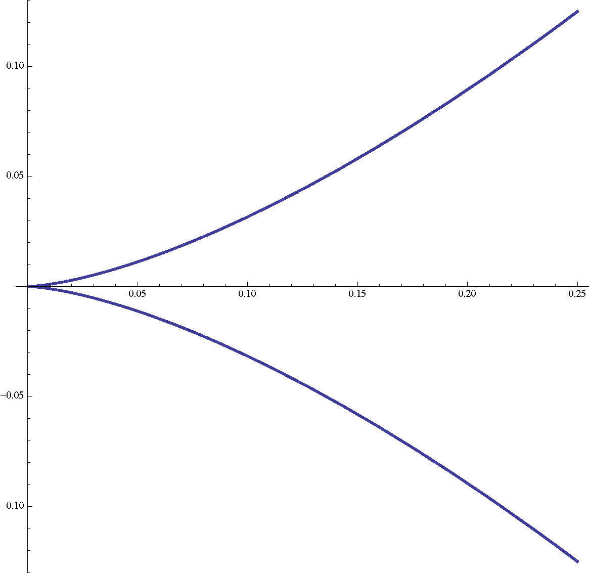
example-curve
But it’s clear that we can write any single-variable function $ f(x)$ in this parametric form: just choose $ x(t) = t$ and $ y(t) = f(t)$. So these are really more general objects than regular old functions (although we’ll only be working with polynomials in this post).
Quickly recapping, a single-parameter polynomial plane curve is defined as a pair of polynomials $ x(t), y(t)$ in the same variable $ t$. Sometimes, if we want to express the whole gadget in one piece, we can take the coefficients of common powers of $ t$ and write them as vectors in the $ x$ and $ y$ parts. Using the $ x(t) = t^2, y(t) = t^3$ example above, we can rewrite it as
$$\mathbf{f}(t) = (0,1) t^3 + (1,0) t^2$$Here the coefficients are points (which are the same as vectors) in the plane, and we represent the function $ f$ in boldface to emphasize that the output is a point. The linear-algebraist might recognize that pairs of polynomials form a vector space, and further combine them as $ (0, t^3) + (t^2, 0) = (t^2, t^3)$. But for us, thinking of points as coefficients of a single polynomial is actually better.
We will also restrict our attention to single-parameter polynomial plane curves for which the variable $ t$ is allowed to range from zero to one. This might seem like an awkward restriction, but in fact every finite single-parameter polynomial plane curve can be written this way (we won’t bother too much with the details of how this is done). For the purpose of brevity, we will henceforth call a “single-parameter polynomial plane curve where $ t$ ranges from zero to one” simply a “curve.”
Now there are some very nice things we can do with curves. For instance, given any two points in the plane $ P = (p_1, p_2), Q = (q_1, q_2)$ we can describe the straight line between them as a curve: $ \mathbf{L}(t) = (1-t)P + tQ$. Indeed, at $ t=0$ the value $ \mathbf{L}(t)$ is exactly $ P$, at $ t=1$ it’s exactly $ Q$, and the equation is a linear polynomial in $ t$. Moreover (without getting too much into the calculus details), the line $ \mathbf{L}$ travels at “unit speed” from $ P$ to $ Q$. In other words, we can think of $ \mathbf{L}$ as describing the motion of a particle from $ P$ to $ Q$ over time, and at time $ 1/4$ the particle is a quarter of the way there, at time $ 1/2$ it’s halfway, etc. (An example of a straight line which doesn’t have unit speed is, e.g. $ (1-t^2) P + t^2 Q$.)
More generally, let’s add a third point $ R$. We can describe a path which goes from $ P$ to $ R$, and is “guided” by $ Q$ in the middle. This idea of a “guiding” point is a bit abstract, but computationally no more difficult. Instead of travelling from one point to another at constant speed, we want to travel from one line to another at constant speed. That is, call the two curves describing lines from $ P \to Q$ and $ Q \to R$ $ \mathbf{L}_1, \mathbf{L_2}$, respectively. Then the curve “guided” by $ Q$ can be written as a curve
$$\displaystyle \mathbf{F}(t) = (1-t)\mathbf{L}_1(t) + t \mathbf{L}_2(t)$$Multiplying this all out gives the formula
$$\displaystyle \mathbf{F}(t) = (1-t)^2 P + 2t(1-t)Q + t^2 R$$We can interpret this again in terms of a particle moving. At the beginning of our curve the value of $ t$ is small, and so we’re sticking quite close to the line $ \mathbf{L}_1$ As time goes on the point $ \mathbf{F}(t)$ moves along the line between the points $ \mathbf{L}_1(t)$ and $ \mathbf{L}_2(t)$, which are themselves moving. This traces out a curve which looks like this
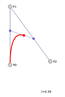
This screenshot was taken from a wonderful demo by data visualization consultant Jason Davies. It expresses the mathematical idea quite superbly, and one can drag the three points around to see how it changes the resulting curve. One should play with it for at least five minutes.
The entire idea of a Bezier curve is a generalization of this principle: given a list $ P_0, \dots, P_n$ of points in the plane, we want to describe a curve which travels from the first point to the last, and is “guided” in between by the remaining points. A Bezier curve is a realization of such a curve (a single-parameter polynomial plane curve) which is the inductive continuation of what we described above: we travel at unit speed from a Bezier curve defined by the first $ n-1$ points in the list to the curve defined by the last $ n-1$ points. The base case is the straight-line segment (or the single point, if you wish). Formally,
Definition: Given a list of points in the plane $ P_0, \dots, P_n$ we define the degree $ n-1$ Bezier curve recursively as
$$\begin{aligned} \mathbf{B}_{P_0}(t) &= P_0 \\\ \mathbf{B}_{P_0 P_1 \dots P_n}(t) &= (1-t)\mathbf{B}_{P_0 P_1 \dots P_{n-1}} + t \mathbf{B}_{P_1P_2 \dots P_n}(t) \end{aligned}$$We call $ P_0, \dots, P_n$ the control points of $ \mathbf{B}$.
While the concept of travelling at unit speed between two lower-order Bezier curves is the real heart of the matter (and allows us true computational insight), one can multiply all of this out (using the formula for binomial coefficients) and get an explicit formula. It is:
$$\displaystyle \mathbf{B}_{P_0 \dots P_n} = \sum_{k=0}^n \binom{n}{k}(1-t)^{n-k}t^k P_k$$And for example, a cubic Bezier curve with control points $ P_0, P_1, P_2, P_3$ would have equation
$$\displaystyle (1-t)^3 P_0 + 3(1-t)^2t P_1 + 3(1-t)t^2 P_2 + t^3 P_3$$Higher dimensional Bezier curves can be quite complicated to picture geometrically. For instance, the following is a fifth-degree Bezier curve (with six control points).
BezierCurve
The additional line segments drawn show the recursive nature of the curve. The simplest are the green points, which travel from control point to control point. Then the blue points travel on the line segments between green points, the pink travel along the line segments between blue, the orange between pink, and finally the red point travels along the line segment between the orange points.
Without the recursive structure of the problem (just seeing the curve) it would be a wonder how one could actually compute with these things. But as we’ll see, the algorithm for drawing a Bezier curve is very natural.
Bezier Curves as Data, and de Casteljau’s Algorithm
Let’s derive and implement the algorithm for painting a Bezier curve to a screen using only the ability to draw straight lines. For simplicity, we’ll restrict our attention to degree-three (cubic) Bezier curves. Indeed, every Bezier curve can be written as a combination of cubic curves via the recursive definition, and in practice cubic curves balance computational efficiency and expressiveness. All of the code we present in this post will be in Javascript, and is available on this blog’s Github page.
So then a cubic Bezier curve is represented in a program by a list of four points. For example,
var curve = [[1,2], [5,5], [4,0], [9,3]];
Most graphics libraries (including the HTML5 canvas standard) provide a drawing primitive that can output Bezier curves given a list of four points. But suppose we aren’t given such a function. Suppose that we only have the ability to draw straight lines. How would one go about drawing an approximation to a Bezier curve? If such an algorithm exists (it does, and we’re about to see it) then we could make the approximation so fine that it is visually indistinguishable from a true Bezier curve.
The key property of Bezier curves that allows us to come up with such an algorithm is the following:
Any cubic Bezier curve $ \mathbf{B}$ can be split into two, end to end, which together trace out the same curve as $ \mathbf{B}$.
Let see exactly how this is done. Let $ \mathbf{B}(t)$ be a cubic Bezier curve with control points $ P_0, P_1, P_2, P_3$, and let’s say we want to split it exactly in half. We notice that the formula for the curve when we plug in $ 1/2$, which is
$$\displaystyle \mathbf{B}(1/2) = \frac{1}{2^3}(P_0 + 3P_1 + 3P_2 + P_3)$$Moreover, our recursive definition gave us a way to evaluate the point in terms of smaller-degree curves. But when these are evaluated at 1/2 their formulae are similarly easy to write down. The picture looks like this:
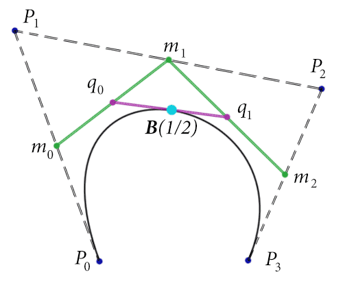
subdivision
The green points are the degree one curves, the pink points are the degree two curves, and the blue point is the cubic curve. We notice that, since each of the curves are evaluated at $ t=1/2$, each of these points can be described as the midpoints of points we already know. So $ m_0 = (P_0 + P_1) / 2, q_0 = (m_0 + m_1)/2$, etc.
In fact, the splitting of the two curves we want is precisely given by these points. That is, the “left” half of the curve is given by the curve $ \mathbf{L}(t)$ with control points $ P_0, m_0, q_0, \mathbf{B}(1/2)$, while the “right” half $ \mathbf{R}(t)$ has control points $ \mathbf{B}(1/2), q_1, m_2, P_3$.
How can we be completely sure these are the same Bezier curves? Well, they’re just polynomials. We can compare them for equality by doing a bunch of messy algebra. But note, since $ \mathbf{L}(t)$ only travels halfway along $ \mathbf{B}(t)$, to check they are the same is to equate $ \mathbf{L}(t)$ with $ \mathbf{B}(t/2)$, since as $ t$ ranges from zero to one, $ t/2$ ranges from zero to one half. Likewise, we can compare $ \mathbf{B}((t+1)/2)$ with $ \mathbf{R}(t)$.
The algebra is very messy, but doable. As a test of this blog’s newest tools, here’s a screen cast of me doing the algebra involved in proving the two curves are identical.
Now that that’s settled, we have a nice algorithm for splitting a cubic Bezier (or any Bezier) into two pieces. In Javascript,
function subdivide(curve) {
   var firstMidpoints = midpoints(curve);
   var secondMidpoints = midpoints(firstMidpoints);
   var thirdMidpoints = midpoints(secondMidpoints);

   return [[curve[0], firstMidpoints[0], secondMidpoints[0], thirdMidpoints[0]],
          [thirdMidpoints[0], secondMidpoints[1], firstMidpoints[2], curve[3]]];
}
Here “curve” is a list of four points, as described at the beginning of this section, and the output is a list of two curves with the correct control points. The “midpoints” function used is quite simple, and we include it here for compelteness:
function midpoints(pointList) {
   var midpoint = function(p, q) {
      return [(p[0] + q[0]) / 2.0, (p[1] + q[1]) / 2.0];
   };

   var midpointList = new Array(pointList.length - 1);
   for (var i = 0; i < midpointList.length; i++) {
      midpointList[i] = midpoint(pointList[i], pointList[i+1]);
   }

   return midpointList;
}
It just accepts as input a list of points and computes their sequential midpoints. So a list of $ n$ points is turned into a list of $ n-1$ points. As we saw, we need to call this function $ d-1$ times to compute the segmentation of a degree $ d$ Bezier curve.
As explained earlier, we can keep subdividing our curve over and over until each of the tiny pieces are basically lines. That is, our function to draw a Bezier curve from the beginning will be as follows:
function drawCurve(curve, context) {
   if (isFlat(curve)) {
      drawSegments(curve, context);
   } else {
      var pieces = subdivide(curve);
      drawCurve(pieces[0], context);
      drawCurve(pieces[1], context);
   }
}
In words, as long as the curve isn’t “flat,” we want to subdivide and draw each piece recursively. If it is flat, then we can simply draw the three line segments of the curve and be reasonably sure that it will be a good approximation. The context variable sitting there represents the canvas to be painted to; it must be passed through to the “drawSegments” function, which simply paints a straight line to the canvas.
Of course this raises the obvious question: how can we tell if a Bezier curve is flat? There are many ways to do so. One could compute the angles of deviation (from a straight line) at each interior control point and add them up. Or one could compute the volume of the enclosed quadrilateral. However, computing angles and volumes is usually not very nice: angles take a long time to compute and volumes have stability issues, and the algorithms which are stable are not very simple. We want a measurement which requires only basic arithmetic and perhaps a few logical conditions to check.
It turns out there is such a measurement. It’s originally attributed to Roger Willcocks, but it’s quite simple to derive by hand.
Essentially, we want to measure the “flatness” of a cubic Bezier curve by computing the distance of the actual curve at time $ t$ from where the curve would be at time $ t$ if the curve were a straight line.
Formally, given $ \mathbf{B}(t)$ with control points $ P_0, P_1, P_2, P_3$ as usual, we can define the straight-line Bezier cubic as the colossal sum
$$\displaystyle \mathbf{S}(t) = (1-t)^3P_0 + 3(1-t)^2t \left ( \frac{2}{3}P_0 + \frac{1}{3}P_3 \right ) + 3(1-t)t^2 \left ( \frac{1}{3}P_0 + \frac{2}{3}P_3 \right ) + t^3 P_3 $$There’s nothing magical going on here. We’re simply giving the Bezier curve with control points $ P_0, \frac{2}{3}P_0 + \frac{1}{3}P_3, \frac{1}{3}P_0 + \frac{2}{3}P_3, P_3$. One should think about this as points which are a 0, 1/3, 2/3, and 1 fraction of the way from $ P_0$ to $ P_3$ on a straight line.
Then we define the function $ d(t) = \left \| \mathbf{B}(t) – \mathbf{S}(t) \right \|$ to be the distance between the two curves at the same time $ t$. The flatness value of $ \mathbf{B}$ is the maximum of $ d$ over all values of $ t$. If this flatness value is below a certain tolerance level, then we call the curve flat.
With a bit of algebra we can simplify this expression. First, the value of $ t$ for which the distance is maximized is the same as when its square is maximized, so we can omit the square root computation at the end and take that into account when choosing a flatness tolerance.
Now lets actually write out the difference as a single polynomial. First, we can cancel the 3’s in $ \mathbf{S}(t)$ and write the polynomial as
$$\displaystyle \mathbf{S}(t) = (1-t)^3 P_0 + (1-t)^2t (2P_0 + P_3) + (1-t)t^2 (P_0 + 2P_3) + t^3 P_3$$and so $ \mathbf{B}(t) – \mathbf{S}(t)$ is (by collecting coefficients of the like terms $ (1-t)^it^j$)
$$\displaystyle (1-t)^2t (3 P_1 – 2P_0 – P_3) + (1-t)t^2 (3P_2 – P_0 – 2P_3) $$Factoring out the $ (1-t)t$ from both terms and setting $ a = 3P_1 – 2P_0 – P_3$, $ b = 3P_2 – P_0 – 2P_3$, we get
$$\displaystyle d^2(t) = \left \| (1-t)t ((1-t)a + tb) \right \|^2 = (1-t)^2t^2 \left \| (1-t)a + tb \right \|^2$$Since the maximum of a product is at most the product of the maxima, we can bound the above quantity by the product of the two maxes. The reason we want to do this is because we can easily compute the two maxes separately. It wouldn’t be hard to compute the maximum without splitting things up, but this way ends up with fewer computational steps for our final algorithm, and the visual result is equally good.
Using some elementary single-variable calculus, the maximum value of $ (1-t)^2t^2$ for $ 0 \leq t \leq 1$ turns out to be $ 1/16$. And the norm of a vector is just the sum of squares of its components. If $ a = (a_x, a_y)$ and $ b = (b_x, b_y)$, then the norm above is exactly
$$\displaystyle ((1-t)a_x + tb_x)^2 + ((1-t)a_y + tb_y)^2$$And notice: for any real numbers $ z, w$ the quantity $ (1-t)z + tw$ is exactly the straight line from $ z$ to $ w$ we know so well. The maximum over all $ t$ between zero and one is obviously the maximum of the endpoints $ z, w$. So the max of our distance function $ d^2(t)$ is bounded by
$$\displaystyle \frac{1}{16} (\textup{max}(a_x^2, b_x^2) + \textup{max}(a_y^2, b_y^2))$$And so our condition for being flat is that this bound is smaller than some allowable tolerance. We may safely factor the 1/16 into this tolerance bound, and so this is enough to write a function.
function isFlat(curve) {
   var tol = 10; // anything below 50 is roughly good-looking

   var ax = 3.0*curve[1][0] - 2.0*curve[0][0] - curve[3][0]; ax *= ax;
   var ay = 3.0*curve[1][1] - 2.0*curve[0][1] - curve[3][1]; ay *= ay;
   var bx = 3.0*curve[2][0] - curve[0][0] - 2.0*curve[3][0]; bx *= bx;
   var by = 3.0*curve[2][1] - curve[0][1] - 2.0*curve[3][1]; by *= by;

   return (Math.max(ax, bx) + Math.max(ay, by) <= tol);
}
And there we have it. We write a simple HTML page to access a canvas element and a few extra helper functions to draw the line segments when the curve is flat enough, and present the final result in this interactive demonstration (you can perturb the control points).
The picture you see on that page (given below) is my rendition of Picasso’s “Dog” drawing as a sequence of nine Bezier curves. I think the resemblance is uncanny.
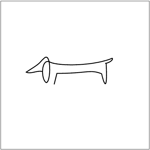
Picasso's 'Dog,' redesigned as a sequence of eight bezier curves.
While we didn’t invent the drawing itself (and hence shouldn’t attach our signature to it), we did come up with the representation as a sequence of Bezier curves. It only seems fitting to present that as the work of art. Here we’ve distilled the representation down to a single file: the first line is the dimension of the canvas, and each subsequent line represents a cubic Bezier curve. Comments are included for readability.
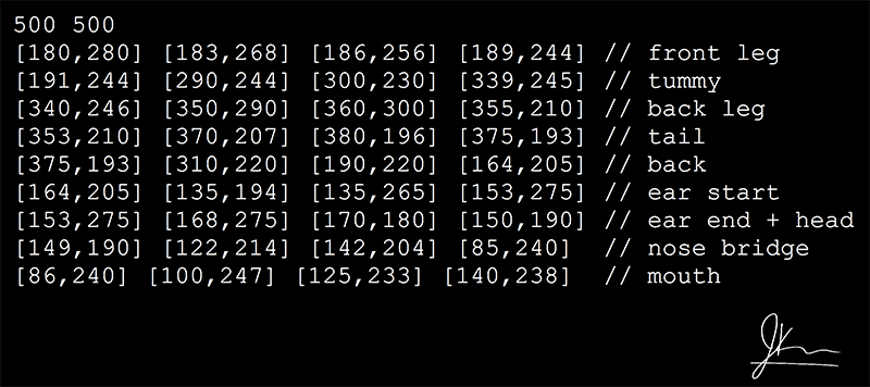
bezier-dog-for-web
We didn’t go as deep into the theory of Bezier curves as we could have. If the reader is itching for more (and a more calculus-based approach), see this lengthy primer. It contains practically everything one could want to know about Bezier curves, with nice interactive demos written in Processing.
Until next time!
Want to respond? Send me an email, post a webmention, or find me elsewhere on the internet.