
startups
The software world is always atwitter with predictions on the next big piece of technology. And a lot of chatter focuses on what venture capitalists express interest in. As an investor, how do you pick a good company to invest in? Do you notice quirky names like “Kaggle” and “Meebo,” require deep technical abilities, or value a charismatic sales pitch?
When it comes to innovation in software engineering and computer science, and that as a society we should value big pushes forward much more than we do. But making safe investments is almost always at odds with innovation. And so every venture capitalist faces the following question. When do you focus investment in those companies that have proven to succeed, and when do you explore new options for growth? A successful venture capitalist must strike a fine balance between this kind of exploration and exploitation. Explore too much and you won’t make enough profit to sustain yourself. Narrow your view too much and you will miss out on opportunities whose return surpasses any of your current prospects.
In life and in business there is no correct answer on what to do, partly because we just don’t have a good understanding of how the world works (or markets, or people, or the weather). In mathematics, however, we can meticulously craft settings that have solid answers. In this post we’ll describe one such scenario, the so-called multi-armed bandit problem, and a simple algorithm called UCB1 which performs close to optimally. Then, in a future post, we’ll analyze the algorithm on some real world data.
As usual, all of the code used in the making of this post are available for download on this blog’s Github page.
Multi-Armed Bandits
The multi-armed bandit scenario is simple to describe, and it boils the exploration-exploitation tradeoff down to its purest form.
Suppose you have a set of $ K$ actions labeled by the integers $ \left \{ 1, 2, \dots, K \right \}$. We call these actions in the abstract, but in our minds they’re slot machines. We can then play a game where, in each round, we choose an action (a slot machine to play), and we observe the resulting payout. Over many rounds, we might explore the machines by trying some at random. Assuming the machines are not identical, we naturally play machines that seem to pay off well more frequently to try to maximize our total winnings.

Exploit away, you lucky ladies.
This is the most general description of the game we could possibly give, and every bandit learning problem has these two components: actions and rewards. But in order to get to a concrete problem that we can reason about, we need to specify more details. Bandit learning is a large tree of variations and this is the point at which the field ramifies. We presently care about two of the main branches.
How are the rewards produced? There are many ways that the rewards could work. One nice option is to have the rewards for action $ i$ be drawn from a fixed distribution $ D_i$ (a different reward distribution for each action), and have the draws be independent across rounds and across actions. This is called the stochastic setting and it’s what we’ll use in this post. Just to pique the reader’s interest, here’s the alternative: instead of having the rewards be chosen randomly, have them be adversarial. That is, imagine a casino owner knows your algorithm and your internal beliefs about which machines are best at any given time. He then fixes the payoffs of the slot machines in advance of each round to screw you up! This sounds dismal, because the casino owner could just make all the machines pay nothing every round. But actually we can design good algorithms for this case, but “good” will mean something different than absolute winnings. And so we must ask:
How do we measure success? In both the stochastic and the adversarial setting, we’re going to have a hard time coming up with any theorems about the performance of an algorithm if we care about how much absolute reward is produced. There’s nothing to stop the distributions from having terrible expected payouts, and nothing to stop the casino owner from intentionally giving us no payout. Indeed, the problem lies in our measurement of success. A better measurement, which we can apply to both the stochastic and adversarial settings, is the notion of regret. We’ll give the definition for the stochastic case, and investigate the adversarial case in a future post.
Definition: Given a player algorithm $ A$ and a set of actions $ \left \{1, 2, \dots, K \right \}$, the cumulative regret of $ A$ in rounds $ 1, \dots, T$ is the difference between the expected reward of the best action (the action with the highest expected payout) and the expected reward of $ A$ for the first $ T$ rounds.
We’ll add some more notation shortly to rephrase this definition in symbols, but the idea is clear: we’re competing against the best action. Had we known it ahead of time, we would have just played it every single round. Our notion of success is not in how well we do absolutely, but in how well we do relative to what is feasible.
Notation
Let’s go ahead and draw up some notation. As before the actions are labeled by integers $ \left \{ 1, \dots, K \right \}$. The reward of action $ i$ is a $ [0,1]$-valued random variable $ X_i$ distributed according to an unknown distribution and possessing an unknown expected value $ \mu_i$. The game progresses in rounds $ t = 1, 2, \dots$ so that in each round we have different random variables $ X_{i,t}$ for the reward of action $ i$ in round $ t$ (in particular, $ X_{i,t}$ and $ X_{i,s}$ are identically distributed). The $ X_{i,t}$ are independent as both $ t$ and $ i$ vary, although when $ i$ varies the distribution changes.
So if we were to play action 2 over and over for $ T$ rounds, then the total payoff would be the random variable $ G_2(T) = \sum_{t=1}^T X_{2,t}$. But by independence across rounds and the linearity of expectation, the expected payoff is just $ \mu_2 T$. So we can describe the best action as the action with the highest expected payoff. Define
$$\displaystyle \mu^* = \max_{1 \leq i \leq K} \mu_i$$We call the action which achieves the maximum $ i^*$.
A policy is a randomized algorithm $ A$ which picks an action in each round based on the history of chosen actions and observed rewards so far. Define $ I_t$ to be the action played by $ A$ in round $ t$ and $ P_i(n)$ to be the number of times we’ve played action $ i$ in rounds $ 1 \leq t \leq n$. These are both random variables. Then the cumulative payoff for the algorithm $ A$ over the first $ T$ rounds, denoted $ G_A(T)$, is just
$$\displaystyle G_A(T) = \sum_{t=1}^T X_{I_t, t}$$and its expected value is simply
$ \displaystyle \mathbb{E}(G_A(T)) = \mu_1 \mathbb{E}(P_1(T)) + \dots + \mu_K \mathbb{E}(P_K(T))$.
Here the expectation is taken over all random choices made by the policy and over the distributions of rewards, and indeed both of these can affect how many times a machine is played.
Now the cumulative regret of a policy $ A$ after the first $ T$ steps, denoted $ R_A(T)$ can be written as
$$\displaystyle R_A(T) = G_{i^*}(T) – G_A(T)$$And the goal of the policy designer for this bandit problem is to minimize the expected cumulative regret, which by linearity of expectation is
$ \mathbb{E}(R_A(T)) = \mu^*T – \mathbb{E}(G_A(T))$.
Before we continue, we should note that there are theorems concerning lower bounds for expected cumulative regret. Specifically, for this problem it is known that no algorithm can guarantee an expected cumulative regret better than $ \Omega(\sqrt{KT})$. It is also known that there are algorithms that guarantee no worse than $ O(\sqrt{KT})$ expected regret. The algorithm we’ll see in the next section, however, only guarantees $ O(\sqrt{KT \log T})$. We present it on this blog because of its simplicity and ubiquity in the field.
The UCB1 Algorithm
The policy we examine is called UCB1, and it can be summed up by the principle of optimism in the face of uncertainty. That is, despite our lack of knowledge in what actions are best we will construct an optimistic guess as to how good the expected payoff of each action is, and pick the action with the highest guess. If our guess is wrong, then our optimistic guess will quickly decrease and we’ll be compelled to switch to a different action. But if we pick well, we’ll be able to exploit that action and incur little regret. In this way we balance exploration and exploitation.
The formalism is a bit more detailed than this, because we’ll need to ensure that we don’t rule out good actions that fare poorly early on. Our “optimism” comes in the form of an upper confidence bound (hence the acronym UCB). Specifically, we want to know with high probability that the true expected payoff of an action $ \mu_i$ is less than our prescribed upper bound. One general (distribution independent) way to do that is to use the Chernoff-Hoeffding inequality.
As a reminder, suppose $ Y_1, \dots, Y_n$ are independent random variables whose values lie in $ [0,1]$ and whose expected values are $ \mu_i$. Call $ Y = \frac{1}{n}\sum_{i}Y_i$ and $ \mu = \mathbb{E}(Y) = \frac{1}{n} \sum_{i} \mu_i$. Then the Chernoff-Hoeffding inequality gives an exponential upper bound on the probability that the value of $ Y$ deviates from its mean. Specifically,
$$\displaystyle \textup{P}(Y + a < \mu) \leq e^{-2na^2}$$For us, the $ Y_i$ will be the payoff variables for a single action $ j$ in the rounds for which we choose action $ j$. Then the variable $ Y$ is just the empirical average payoff for action $ j$ over all the times we’ve tried it. Moreover, $ a$ is our one-sided upper bound (and as a lower bound, sometimes). We can then solve this equation for $ a$ to find an upper bound big enough to be confident that we’re within $ a$ of the true mean.
Indeed, if we call $ n_j$ the number of times we played action $ j$ thus far, then $ n = n_j$ in the equation above, and using $ a = a(j,T) = \sqrt{2 \log(T) / n_j}$ we get that $ \textup{P}(Y > \mu + a) \leq T^{-4}$, which converges to zero very quickly as the number of rounds played grows. We’ll see this pop up again in the algorithm’s analysis below. But before that note two things. First, assuming we don’t play an action $ j$, its upper bound $ a$ grows in the number of rounds. This means that we never permanently rule out an action no matter how poorly it performs. If we get extremely unlucky with the optimal action, we will eventually be convinced to try it again. Second, the probability that our upper bound is wrong decreases in the number of rounds independently of how many times we’ve played the action. That is because our upper bound $ a(j, T)$ is getting bigger for actions we haven’t played; any round in which we play an action $ j$, it must be that $ a(j, T+1) = a(j,T)$, although the empirical mean will likely change.
With these two facts in mind, we can formally state the algorithm and intuitively understand why it should work.
UCB1: Play each of the $ K$ actions once, giving initial values for empirical mean payoffs $ \overline{x}_i$ of each action $ i$. For each round $ t = K, K+1, \dots$:
Let $ n_j$ represent the number of times action $ j$ was played so far. Play the action $ j$ maximizing $ \overline{x}_j + \sqrt{2 \log t / n_j}$. Observe the reward $ X_{j,t}$ and update the empirical mean for the chosen action.
And that’s it. Note that we’re being super stateful here: the empirical means $ x_j$ change over time, and we’ll leave this update implicit throughout the rest of our discussion (sorry, functional programmers, but the notation is horrendous otherwise).
Before we implement and test this algorithm, let’s go ahead and prove that it achieves nearly optimal regret. The reader uninterested in mathematical details should skip the proof, but the discussion of the theorem itself is important. If one wants to use this algorithm in real life, one needs to understand the guarantees it provides in order to adequately quantify the risk involved in using it.
Theorem: Suppose that UCB1 is run on the bandit game with $ K$ actions, each of whose reward distribution $ X_{i,t}$ has values in [0,1]. Then its expected cumulative regret after $ T$ rounds is at most $ O(\sqrt{KT \log T})$.
Actually, we’ll prove a more specific theorem. Let $ \Delta_i$ be the difference $ \mu^* – \mu_i$, where $ \mu^*$ is the expected payoff of the best action, and let $ \Delta$ be the minimal nonzero $ \Delta_i$. That is, $ \Delta_i$ represents how suboptimal an action is and $ \Delta$ is the suboptimality of the second best action. These constants are called problem-dependent constants. The theorem we’ll actually prove is:
Theorem: Suppose UCB1 is run as above. Then its expected cumulative regret $ \mathbb{E}(R_{\textup{UCB1}}(T))$ is at most
$$\displaystyle 8 \sum_{i : \mu_i < \mu^*} \frac{\log T}{\Delta_i} + \left ( 1 + \frac{\pi^2}{3} \right ) \left ( \sum_{j=1}^K \Delta_j \right )$$Okay, this looks like one nasty puppy, but it’s actually not that bad. The first term of the sum signifies that we expect to play any suboptimal machine about a logarithmic number of times, roughly scaled by how hard it is to distinguish from the optimal machine. That is, if $ \Delta_i$ is small we will require more tries to know that action $ i$ is suboptimal, and hence we will incur more regret. The second term represents a small constant number (the $ 1 + \pi^2 / 3$ part) that caps the number of times we’ll play suboptimal machines in excess of the first term due to unlikely events occurring. So the first term is like our expected losses, and the second is our risk.
But note that this is a worst-case bound on the regret. We’re not saying we will achieve this much regret, or anywhere near it, but that UCB1 simply cannot do worse than this. Our hope is that in practice UCB1 performs much better.
Before we prove the theorem, let’s see how derive the $ O(\sqrt{KT \log T})$ bound mentioned above. This will require familiarity with multivariable calculus, but such things must be endured like ripping off a band-aid. First consider the regret as a function $ R(\Delta_1, \dots, \Delta_K)$ (excluding of course $ \Delta^*$), and let’s look at the worst case bound by maximizing it. In particular, we’re just finding the problem with the parameters which screw our bound as badly as possible, The gradient of the regret function is given by
$$\displaystyle \frac{\partial R}{\partial \Delta_i} = – \frac{8 \log T}{\Delta_i^2} + 1 + \frac{\pi^2}{3}$$and it’s zero if and only if for each $ i$, $ \Delta_i = \sqrt{\frac{8 \log T}{1 + \pi^2/3}} = O(\sqrt{\log T})$. However this is a minimum of the regret bound (the Hessian is diagonal and all its eigenvalues are positive). Plugging in the $ \Delta_i = O(\sqrt{\log T})$ (which are all the same) gives a total bound of $ O(K \sqrt{\log T})$. If we look at the only possible endpoint (the $ \Delta_i = 1$), then we get a local maximum of $ O(K \sqrt{\log T})$. But this isn’t the $ O(\sqrt{KT \log T})$ we promised, what gives? Well, this upper bound grows arbitrarily large as the $ \Delta_i$ go to zero. But at the same time, if all the $ \Delta_i$ are small, then we shouldn’t be incurring much regret because we’ll be picking actions that are close to optimal!
Indeed, if we assume for simplicity that all the $ \Delta_i = \Delta$ are the same, then another trivial regret bound is $ \Delta T$ (why?). The true regret is hence the minimum of this regret bound and the UCB1 regret bound: as the UCB1 bound degrades we will eventually switch to the simpler bound. That will be a non-differentiable switch (and hence a critical point) and it occurs at $ \Delta = O(\sqrt{(K \log T) / T})$. Hence the regret bound at the switch is $ \Delta T = O(\sqrt{KT \log T})$, as desired.
Proving the Worst-Case Regret Bound
Proof. The proof works by finding a bound on $ P_i(T)$, the expected number of times UCB chooses an action up to round $ T$. Using the $ \Delta$ notation, the regret is then just $ \sum_i \Delta_i \mathbb{E}(P_i(T))$, and bounding the $ P_i$’s will bound the regret.
Recall the notation for our upper bound $ a(j, T) = \sqrt{2 \log T / P_j(T)}$ and let’s loosen it a bit to $ a(y, T) = \sqrt{2 \log T / y}$ so that we’re allowed to “pretend” a action has been played $ y$ times. Recall further that the random variable $ I_t$ has as its value the index of the machine chosen. We denote by $ \chi(E)$ the indicator random variable for the event $ E$. And remember that we use an asterisk to denote a quantity associated with the optimal action (e.g., $ \overline{x}^*$ is the empirical mean of the optimal action).
Indeed for any action $ i$, the only way we know how to write down $ P_i(T)$ is as
$$\displaystyle P_i(T) = 1 + \sum_{t=K}^T \chi(I_t = i)$$The 1 is from the initialization where we play each action once, and the sum is the trivial thing where just count the number of rounds in which we pick action $ i$. Now we’re just going to pull some number $ m-1$ of plays out of that summation, keep it variable, and try to optimize over it. Since we might play the action fewer than $ m$ times overall, this requires an inequality.
$$P_i(T) \leq m + \sum_{t=K}^T \chi(I_t = i \textup{ and } P_i(t-1) \geq m)$$These indicator functions should be read as sentences: we’re just saying that we’re picking action $ i$ in round $ t$ and we’ve already played $ i$ at least $ m$ times. Now we’re going to focus on the inside of the summation, and come up with an event that happens at least as frequently as this one to get an upper bound. Specifically, saying that we’ve picked action $ i$ in round $ t$ means that the upper bound for action $ i$ exceeds the upper bound for every other action. In particular, this means its upper bound exceeds the upper bound of the best action (and $ i$ might coincide with the best action, but that’s fine). In notation this event is
$$\displaystyle \overline{x}_i + a(P_i(t), t-1) \geq \overline{x}^* + a(P^*(T), t-1)$$Denote the upper bound $ \overline{x}_i + a(i,t)$ for action $ i$ in round $ t$ by $ U_i(t)$. Since this event must occur every time we pick action $ i$ (though not necessarily vice versa), we have
$$\displaystyle P_i(T) \leq m + \sum_{t=K}^T \chi(U_i(t-1) \geq U^*(t-1) \textup{ and } P_i(t-1) \geq m)$$We’ll do this process again but with a slightly more complicated event. If the upper bound of action $ i$ exceeds that of the optimal machine, it is also the case that the maximum upper bound for action $ i$ we’ve seen after the first $ m$ trials exceeds the minimum upper bound we’ve seen on the optimal machine (ever). But on round $ t$ we don’t know how many times we’ve played the optimal machine, nor do we even know how many times we’ve played machine $ i$ (except that it’s more than $ m$). So we try all possibilities and look at minima and maxima. This is a pretty crude approximation, but it will allow us to write things in a nicer form.
Denote by $ \overline{x}_{i,s}$ the random variable for the empirical mean after playing action $ i$ a total of $ s$ times, and $ \overline{x}^*_s$ the corresponding quantity for the optimal machine. Realizing everything in notation, the above argument proves that
$$\displaystyle P_i(T) \leq m + \sum_{t=K}^T \chi \left ( \max_{m \leq s < t} \overline{x}_{i,s} + a(s, t-1) \geq \min_{0 < s’ < t} \overline{x}^*_{s’} + a(s’, t-1) \right )$$Indeed, at each $ t$ for which the max is greater than the min, there will be at least one pair $ s,s’$ for which the values of the quantities inside the max/min will satisfy the inequality. And so, even worse, we can just count the number of pairs $ s, s’$ for which it happens. That is, we can expand the event above into the double sum which is at least as large:
$$\displaystyle P_i(T) \leq m + \sum_{t=K}^T \sum_{s = m}^{t-1} \sum_{s’ = 1}^{t-1} \chi \left ( \overline{x}_{i,s} + a(s, t-1) \geq \overline{x}^*_{s’} + a(s’, t-1) \right )$$We can make one other odd inequality by increasing the sum to go from $ t=1$ to $ \infty$. This will become clear later, but it means we can replace $ t-1$ with $ t$ and thus have
$$\displaystyle P_i(T) \leq m + \sum_{t=1}^\infty \sum_{s = m}^{t-1} \sum_{s’ = 1}^{t-1} \chi \left ( \overline{x}_{i,s} + a(s, t) \geq \overline{x}^*_{s’} + a(s’, t) \right )$$Now that we’ve slogged through this mess of inequalities, we can actually get to the heart of the argument. Suppose that this event actually happens, that $ \overline{x}_{i,s} + a(s, t) \geq \overline{x}^*_{s’} + a(s’, t)$. Then what can we say? Well, consider the following three events:
(1) $ \displaystyle \overline{x}^*_{s’} \leq \mu^* – a(s’, t)$ (2) $ \displaystyle \overline{x}_{i,s} \geq \mu_i + a(s, t)$ (3) $ \displaystyle \mu^* < \mu_i + 2a(s, t)$
In words, (1) is the event that the empirical mean of the optimal action is less than the lower confidence bound. By our Chernoff bound argument earlier, this happens with probability $ t^{-4}$. Likewise, (2) is the event that the empirical mean payoff of action $ i$ is larger than the upper confidence bound, which also occurs with probability $ t^{-4}$. We will see momentarily that (3) is impossible for a well-chosen $ m$ (which is why we left it variable), but in any case the claim is that one of these three events must occur. For if they are all false, we have
$$\displaystyle \begin{matrix} \overline{x}_{i,s} + a(s, t) \geq \overline{x}^*_{s’} + a(s’, t) & > & \mu^* – a(s’,t) + a(s’,t) = \mu^* \\\ \textup{assumed} & (1) \textup{ is false} & \\\ \end{matrix}$$and
$$\begin{matrix} \mu_i + 2a(s,t) & > & \overline{x}_{i,s} + a(s, t) \geq \overline{x}^*_{s’} + a(s’, t) \\\ & (2) \textup{ is false} & \textup{assumed} \\\ \end{matrix}$$But putting these two inequalities together gives us precisely that (3) is true:
$$\mu^* < \mu_i + 2a(s,t)$$This proves the claim.
By the union bound, the probability that at least one of these events happens is $ 2t^{-4}$ plus whatever the probability of (3) being true is. But as we said, we’ll pick $ m$ to make (3) always false. Indeed $ m$ depends on which action $ i$ is being played, and if $ s \geq m > 8 \log T / \Delta_i^2$ then $ 2a(s,t) \leq \Delta_i$, and by the definition of $ \Delta_i$ we have
$ \mu^* – \mu_i – 2a(s,t) \geq \mu^* – \mu_i – \Delta_i = 0$.
Now we can finally piece everything together. The expected value of an event is just its probability of occurring, and so
$$\displaystyle \begin{aligned} \mathbb{E}(P_i(T)) & \leq m + \sum_{t=1}^\infty \sum_{s=m}^t \sum_{s’ = 1}^t \textup{P}(\overline{x}_{i,s} + a(s, t) \geq \overline{x}^*_{s’} + a(s’, t)) \\\ & \leq \left \lceil \frac{8 \log T}{\Delta_i^2} \right \rceil + \sum_{t=1}^\infty \sum_{s=m}^t \sum_{s’ = 1}^t 2t^{-4} \\\ & \leq \frac{8 \log T}{\Delta_i^2} + 1 + \sum_{t=1}^\infty \sum_{s=1}^t \sum_{s’ = 1}^t 2t^{-4} \\\ & = \frac{8 \log T}{\Delta_i^2} + 1 + 2 \sum_{t=1}^\infty t^{-2} \\\ & = \frac{8 \log T}{\Delta_i^2} + 1 + \frac{\pi^2}{3} \\\ \end{aligned}$$The second line is the Chernoff bound we argued above, the third and fourth lines are relatively obvious algebraic manipulations, and the last equality uses the classic solution to Basel’s problem. Plugging this upper bound in to the regret formula we gave in the first paragraph of the proof establishes the bound and proves the theorem.
$$\square$$Implementation and an Experiment
The algorithm is about as simple to write in code as it is in pseudocode. The confidence bound is trivial to implement (though note we index from zero):
def upperBound(step, numPlays):
   return math.sqrt(2 * math.log(step + 1) / numPlays)
And the full algorithm is quite short as well. We define a function ucb1, which accepts as input the number of actions and a function reward which accepts as input the index of the action and the time step, and draws from the appropriate reward distribution. Then implementing ucb1 is simply a matter of keeping track of empirical averages and an argmax. We implement the function as a Python generator, so one can observe the steps of the algorithm and keep track of the confidence bounds and the cumulative regret.
def ucb1(numActions, reward):
   payoffSums = [0] * numActions
   numPlays = [1] * numActions
   ucbs = [0] * numActions

   # initialize empirical sums
   for t in range(numActions):
      payoffSums[t] = reward(t,t)
      yield t, payoffSums[t], ucbs

   t = numActions

   while True:
      ucbs = [payoffSums[i] / numPlays[i] + upperBound(t, numPlays[i]) for i in range(numActions)]
      action = max(range(numActions), key=lambda i: ucbs[i])
      theReward = reward(action, t)
      numPlays[action] += 1
      payoffSums[action] += theReward

      yield action, theReward, ucbs
      t = t + 1
The heart of the algorithm is the second part, where we compute the upper confidence bounds and pick the action maximizing its bound.
We tested this algorithm on synthetic data. There were ten actions and a million rounds, and the reward distributions for each action were uniform from $ [0,1]$, biased by $ 1/k$ for some $ 5 \leq k \leq 15$. The regret and theoretical regret bound are given in the graph below.
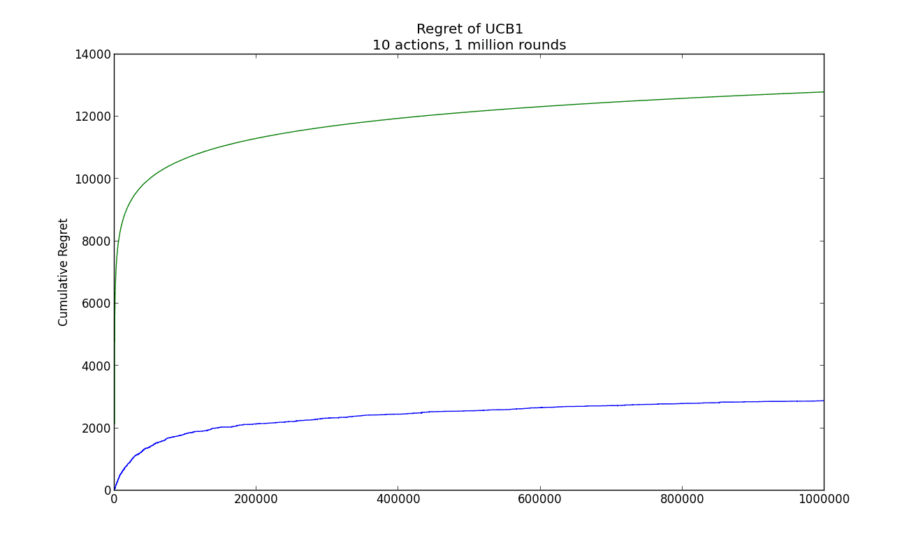
ucb1-simple-example
Note that both curves are logarithmic, and that the actual regret is quite a lot smaller than the theoretical regret. The code used to produce the example and image are available on this blog’s Github page.
Next Time
One interesting assumption that UCB1 makes in order to do its magic is that the payoffs are stochastic and independent across rounds. Next time we’ll look at an algorithm that assumes the payoffs are instead adversarial, as we described earlier. Surprisingly, in the adversarial case we can do about as well as the stochastic case. Then, we’ll experiment with the two algorithms on a real-world application.
Until then!
Want to respond? Send me an email, post a webmention, or find me elsewhere on the internet.