So far in this series we’ve seen two nontrivial algorithms for bandit learning in two different settings. The first was the UCB1 algorithm, which operated under the assumption that the rewards for the trials were independent and stochastic. That is, each slot machine was essentially a biased coin flip, and the algorithm was trying to find the machine with the best odds. The second was the Exp3 algorithm, which held the belief that the payoffs were arbitrary. In particular this includes the possibility that an adversary is setting the payoffs against you, and so we measured the success of an algorithm in terms of how it fares against the best single action (just as we did with UCB1, but with Exp3 it’s a nontrivial decision).
Before we move on to other bandit settings it’s natural to try to experiment with the ones we have on real world data. On one hand it’s interesting to see how they fare outside academia. And more relevantly to the design of the future bandit algorithms we’ll see on this blog, we need to know what worldly problems actually provide in terms of inputs to our learning algorithm in each round.
But another interesting issue goes like this. In the real world we can’t ever really know whether the rewards of the actions are stochastic or adversarial. Many people believe that adversarial settings are far too pathological to be realistic, while others claim that the assumptions made by stochastic models are too strict. To weigh in on this dispute, we’ll dip into a bit of experimental science and see which of the two algorithms performs better on the problem of stock trading. The result is then evidence that stocks behave stochastically or adversarially. But we don’t want to stir up too many flames, so we can always back up behind the veil of applied mathematics (“this model is too simple anyway”).
Indeed the model we use in this post is rather simplistic. I don’t know as much as I should (or as my father would have me know) about stock markets. In fact, I’m more partial to not trade stocks on principle. But I must admit that average-quality stock data is easy to come by, and the basic notions of market interactions lend themselves naturally to many machine learning problems. If the reader has any ideas about how to strengthen the model, I welcome suggestions in the comments (or a fork on github).
A fair warning to the reader, we do not solve the problem of trading stocks by any means. We use a model that’s almost entirely unrealistic, and the results aren’t even that good. I’m quite nervous to publish this at all, just because above all else it reveals my gaping ignorance on how stock markets work. But this author believes in revealing ignorance as learning, if for nothing else than that it provides extremely valuable insight into the nature of a problem and an appreciation of its complexity. So criticize away, dear readers.
As usual, all of the code and data we use in this post is available on this blog’s Github page. Our language of choice for this post is Python.

This little trader got lucky.
Stocks for Dummies (me)
A quick primer on stocks, which is only as detailed as it needs to be for this post: a stock is essentially the sum of the value of all the assets of a company. A publicly traded company divides their stock into a number of “shares,” and owning a share represents partial ownership of the company. If you own 50% of the shares, you own 50% of the company. Companies sell shares or give them to employees as benefits (or options), and use the money gained through their sale for whatever they see fit. The increase in the price of a stock generally signifies the company is successful and growing; for example, stocks generally rise when a hotly anticipated product is announced.
The stock of a company is traded through one of a number of markets called *stock exchanges. The buying and selling interactions are recorded and public, and there are many people in the world who monitor the interactions as they happen (via television, or programmatically) in the hopes of noticing opportunities before others and capitalizing on them. Each interaction induces a change on the price of a share of stock: whenever a share is bought at a certain price, that is the established and recorded price of a share (up to some fudging by brokers which is entirely mysterious to me). In any case, the prices go up and down, and they’re often bundled into “bars” which summarize the data over a certain period of time. The bars we use in this post are daily, and consist of four numbers: the open, the price at the beginning of the day, the high and low, which are self-explanatory, and the close, which is the price at the end of the day.
Bandits and Daily Stock Trading
Now let’s simplify things as much as possible. Our bandit learning algorithm will interact with the market as follows: each day it chooses whether or not to buy a single dollar’s worth of a stock, and at the end of the day it sells the stock and observes the profit. There are no brokers involved, and the price the algorithm sees is the price it gets. In bandit language: the stocks represent actions, and the amount of profit at the end of a day constitutes the payoff of an action in one round. Since small-scale stock price movement is generally very poorly understood, it makes some level of sense to assume the price movements within a given day are adversarial. On the other hand, since we understand them so poorly, we might be tempted to just call them “random” fluctuations, i.e. stochastic. So this is a nice little testbed for seeing which assumption yields a more successful algorithm.
Unlike the traditional image of stock trading where an individual owns shares of a stock over a long period of time, our program will operate on a daily time scale, and hence cannot experience the typical kinds of growth. Nevertheless, we can try to make some money over time, and if it’s a good strategy, we could scale up the single dollar to whatever we’re willing to risk. Specifically, the code we used to compute the payoff is
def payoff(stockTable, t, stock, amountToInvest=1.0):
   openPrice, closePrice = stockTable[stock][t]

   sharesBought = amountToInvest / openPrice
   amountAfterSale = sharesBought * closePrice

   return amountAfterSale - amountToInvest
The remainder of the code is interfacing with the Exp3 and UCB1 functions we gave in previous posts, and data shuffling. We got our data from Google Finance, and we provide it, along with all of the code used in the making of this post, on this blog’s Github page. Before we run our experiments, let’s give a few reasons why this model is unrealistic.
- We assume we can buy/sell fractional shares of a stock, which to my knowledge is not possible. Though this experiment could be redone where you buy a single share of a stock, or with mutual funds/currency exchange/whatever replacing stocks, we didn’t do it this way.
- Brokerage fees can drastically change the success of an algorithm which trades frequently.
- Open and close prices are not typical prices. People will often make decisions based on the time of day, but then again we might expect this to be just another reason that Exp3 would perform better than UCB1.
- We’re not actually trading in the stock market, and so we’re ignoring the effects of our own algorithm on the prices in the market.
- It’s impossible to guarantee you get to use the opening price and closing price in your transactions.
- UCB1 and Exp3 don’t use all of the information available. Indeed, they assume that they would not be able to see the outcome of an action they did not take, but with stocks you can get a good estimate of how much money you would have made had you chosen a different stock.
- Each trial in a bandit learning problem is identical from the learner’s perspective, but one often keeps a stock around while making other decisions.
We’ll come back to #6 after seeing the raw experiments for an unaltered UCB1 and Exp3, because there is a natural extension of the algorithm to handle additional information. I’m sure there are other glaring issues with the experimental setup, and the reader should feel free to rant about it in the comments. It won’t stop me from running the algorithm and seeing what happens just for fun.
Data Sets
We ran the experiment on two sets of stocks. The first set consisted of nine random stocks, taken from the random stocks twitter feed, with 5 years of past data. The stocks are:
lxrx, keg, cuba, tdi, brks, mux, cadx, belfb, htr
And you can view more information about these particular stocks via Google Finance. The second set was a non-random choice of nine Fortune 500 companies with 10 years of past data. The stocks were
amzn, cost, jpm, gs, wfc, msft, tgt, aapl, wmt
And again more information about these stocks is available via Google Finance. For the record, here were the cumulative payoffs of each of the nine Fortune 500 companies:
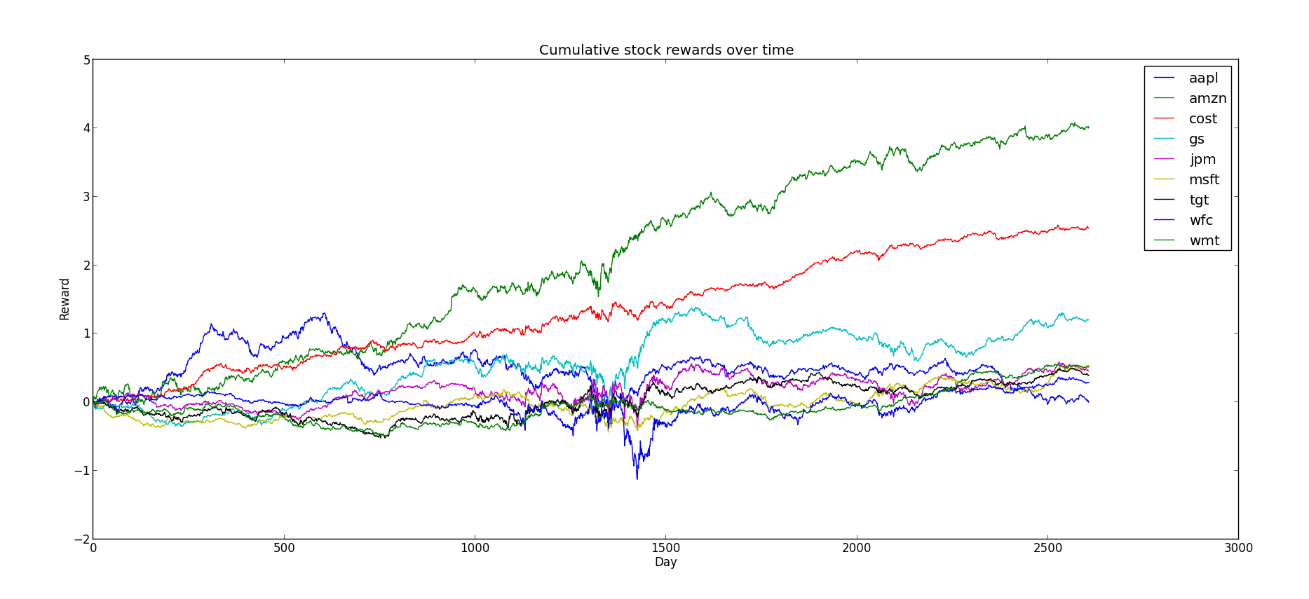
f500-cumulative-rewards
Interestingly, the company which started off with the best prospects (Apple), turned out to have the worst cumulative reward by the end. The long-term winners in our little imaginary world happen to be Amazon, Costco, and Goldman Sachs. Perhaps this gives credence to the assumption that payoffs are adversarial. A learner can easily get tricked into putting too much faith in one action early on.
And for the random stocks:
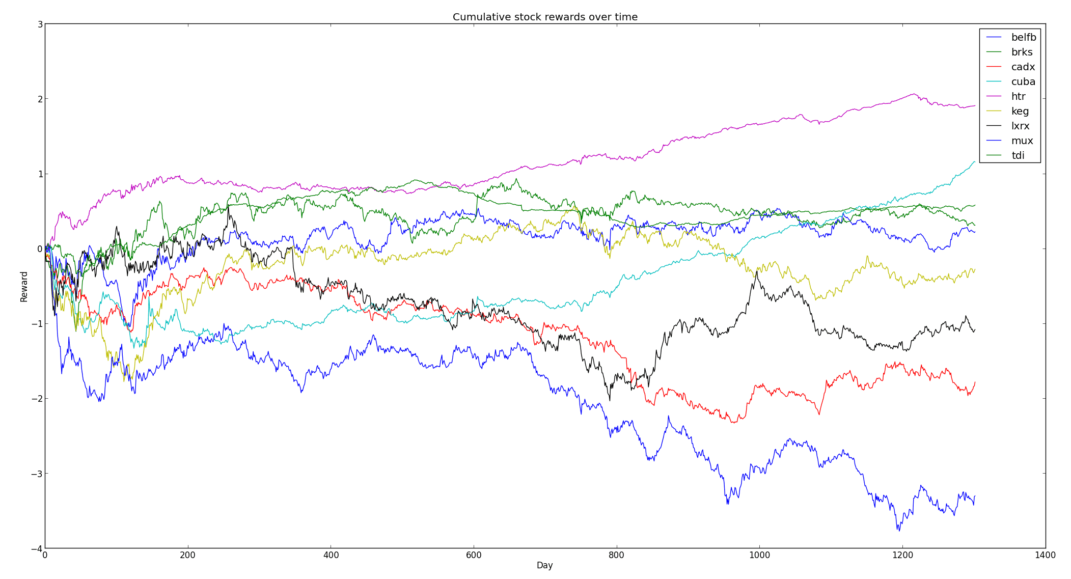
The cumulative payoff for the nine randomly chosen stocks.
The random stocks clearly perform worse and more variably overall (although HTR surpasses most of the Fortune 500 companies, despite its otherwise relatively modest stock growth over the last five years). To my untrained eyes these movements look more like a stochastic model than an adversarial one.
Experiments
Here is a typical example of a run of Exp3 on the Fortune 500 data set (using $ \gamma = 0.33$, recall $ \gamma$ measures the amount of uniform exploration performed):
(Expected payoff, variance) over 1000 trials is (1.122463919564572, 0.5518037498918705)
For a single run:
Payoff was 1.12
Regret was 2.91
Best stock was amzn at 4.02
weights: '0.00, 0.00, 0.00, 0.46, 0.52, 0.00, 0.00, 0.00, 0.01'
And one for UCB1:
(Expected payoff, variance) over 1000 trials is (1.1529891576139333, 0.5012825847001482)
For a single run:
Payoff was 1.73
Regret was 2.29
Best stock was amzn at 4.02
ucbs: '0.234, 0.234, 0.234, 0.234, 0.234, 0.234, 0.234, 0.234, 0.234'
The results are quite curious. Indeed, the expected payoff seems to be a whopping 110% return! The variance of these results is quite high, and so it’s not at all impossible that the algorithm could have a negative return. But just as often it would return around 200% profit.
Before we go risking all our money on this strategy, let’s take a closer look at what’s happening in the algorithm. It appears that for UCB1 the upper confidence bounds assigned to each action are the same! In other words, even after ten years of trials, no single stock “shined” above the others in the eyes of UCB1. It may seem that Exp3 has a leg up on UCB1 in this respect, because it’s clear that it gives higher weights to some stocks over others. However, running the algorithm multiple times shows drastically different weight distributions, and if we average the resulting weights over a thousand rounds, we see that they all have roughly the same mean and variance (the mean being first in the pair):
weight stats for msft: (0.107, 0.025)
weight stats for jpm: (0.109, 0.027)
weight stats for tgt: (0.110, 0.029)
weight stats for gs: (0.112, 0.025)
weight stats for wmt: (0.110, 0.027)
weight stats for aapl: (0.111, 0.027)
weight stats for amzn: (0.120, 0.029)
weight stats for cost: (0.113, 0.026)
weight stats for wfc: (0.107, 0.023)
Indeed, the best stock, Amazon, had an average weight just barely larger (and more variable) than any of the other stocks. So this evidence points to the conclusion that neither EXP3 nor UCB1 has any clue which stock is better. Pairing this with the fact that both algorithms nevertheless perform well would suggest that a random choice of action at each step is equally likely to do well. Indeed, when we run with a “random bandit” that just chooses actions uniformly at random, we get the following results:
(Expected payoff, variance) over 1000 trials is (1.1094227056931132, 0.4403783017367529)
For a single run:
Payoff was 3.13
Regret was 0.90
Best stock was amzn at 4.02
It’s not quite as good as either Exp3 or UCB1, but it’s close and less variable, which means a lot to an investor. In other words, it’s starting to look like Exp3 and UCB1 aren’t doing significantly better than random at all, and that a monkey would do well in this system (for these particular stocks).
Of course, Fortune 500 companies are pretty successful by definition, so let’s turn our attention to the random stocks:
For the random bandit learner:
(Expected payoff, variance) over 1000 trials is (-0.23952295977625776, 1.0787311145181104)
For a single run:
Payoff was -2.01
Regret was 3.92
Best stock was htr at 1.91
For UCB1:
(Expected payoff, variance) over 1000 trials is (-0.3503593899029112, 1.1136234992964154)
For a single run:
Payoff was 0.26
Regret was 1.65
Best stock was htr at 1.91
ucbs: '0.315, 0.315, 0.315, 0.316, 0.315, 0.315, 0.315, 0.315, 0.316'
And for Exp3:
(Expected payoff, variance) over 1000 trials is (-0.25827976810345593, 1.2946101887058519)
For a single run:
Payoff was -0.34
Regret was 2.25
Best stock was htr at 1.91
weights: '0.08, 0.00, 0.14, 0.06, 0.48, 0.00, 0.00, 0.04, 0.19'
But again Exp3 has no idea what stocks are actually best, with the average, variance over 1000 trials being:
weight stats for lxrx: '0.11, 0.02'
weight stats for keg: '0.11, 0.02'
weight stats for htr: '0.12, 0.02'
weight stats for cadx: '0.10, 0.02'
weight stats for belfb: '0.11, 0.02'
weight stats for tdi: '0.11, 0.02'
weight stats for cuba: '0.11, 0.02'
weight stats for mux: '0.11, 0.02'
weight stats for brks: '0.11, 0.02'
The long and short of it is that the choice of Fortune 500 stocks was inherently so biased toward success than a monkey could have made money investing in them, while the average choice of stocks had, if anything, a bias toward loss. And unfortunately using an algorithm like UCB1 or Exp3 straight out of the box doesn’t produce anything better than a monkey.
Issues and Improvements
There are two glaring theoretical issues here that we haven’t yet addressed. One of these goes back to issue #5 in that list we gave at the beginning of the post: the bandit algorithms are assuming they have less information than they actually have! Indeed, at the end of a day of stock trading, you have a good idea what would have happened to you had you bought a different stock, and in our simplified world you can know exactly what your profit would have been. Recalling that UCB1 and Exp3 both maintained some numbers representing the strength of an action (Exp3 had a “weight” and UCB1 an upper confidence bound), the natural extension to both UCB1 and Exp3 is simply to modify the beliefs about all actions after any given round. This is a pretty simple improvement to make in our implementation, since it just changes a single weight update to a loop. For Exp3:
for choice in range(numActions):
   rewardForUpdate = reward(choice, t)
   scaledReward = (rewardForUpdate - rewardMin) / (rewardMax - rewardMin)
   estimatedReward = 1.0 * scaledReward / probabilityDistribution[choice]
   weights[choice] *= math.exp(estimatedReward * gamma / numActions)
With a similar loop for UCB1. This code should be familiar from our previous posts on bandits. We then rerun the new algorithms on the same data sets, and the results are somewhat surprising. First, UCB1 on Fortune 500:
(Expected payoff, variance) over 1000 trials is (3.530670654982728, 0.007713190816014095)
For a single run:
Payoff was 3.56
Regret was 0.47
This is clearly outperforming the random bandit learning algorithm, with an average return of 350%! In fact, it does almost as well as the best stock, and the variance is quite low. UCB1 also outperforms Exp3, which fares comparably to its pre-improved self. That is, it’s still not much better than random:
(Expected payoff, variance) over 1000 trials is (1.1424797906901956, 0.434335471375294)
For a single run:
Payoff was 1.24
Regret was 2.79
And also for the random stocks, UCB1 with improvements outperforms Exp3 and UCB1 without improvements. UCB1:
(Expected payoff, variance) over 1000 trials is (0.680211923900068, 0.04226672915962647)
For a single run:
Payoff was 0.82
Regret was 1.09
And Exp3:
(Expected payoff, variance) over 1000 trials is (-0.2242152508929378, 1.1312843329929194)
For a single run:
Payoff was -0.16
Regret was 2.07
We might wonder why this is the case, and there is a plausible explanation. See, Exp3 has a difficult life: it has to assume that at any time the adversary can completely change the game. And so Exp3 must remain vigilant, continuing to try options it knows to be terrible for fear that they may spontaneously do well. Exp3 is the grandfather who, after 75 years of not winning the lotto, continues to buy tickets every week. A better analogy might be a lioness who, even after being moved to the zoo, stays up all night to protect a cub from predators. This gives us quite a new perspective on Exp3: the world really has to be that messed up for Exp3 to be useful. As we saw, UCB1 is much more eager to jump on a winning bandwagon, and it paid off in both the good (Fortune 500) and bad (random stock) scenarios. All in all, this experiment would provide some minor evidence that the stock market (or just this cheesy version of it) is more stochastic than adversarial.
The second problem is that we’re treating these stocks as if they were isolated from the rest of the world. Indeed, along with each stock comes some kind of context in the form of information about that stock. Historical prices, corporate announcements, cyclic boom and bust, what the talking heads think, all of this may be relevant to the price fluctuations of a stock on any given day. While Exp3 and UCB1 are ill-equipped to handle such a rich landscape, researchers in bandit learning have recognized the importance of context in decision making. So much so, in fact, that an entire subfield of “Contextual Bandits” was born. John Langford, perhaps the world’s leading expert on bandit learning, wrote on his blog in 2007,
I’m having difficulty finding interesting real-world k-Armed Bandit settings which aren’t better thought of as Contextual Bandits in practice. For myself, bandit algorithms are (at best) motivational because they can not be applied to real-world problems without altering them to take context into account.
I tend to agree with him. Bandit problems almost always come with some inherent additional structure in the real world, and the best algorithms will always take advantage of that structure. A “context” associated with each round is perhaps the weakest kind of structure, so it’s a natural place to look for better algorithms.
So that’s what we’ll do in the future of this series. But before then we might decide to come up with another experiment to run Exp3 and UCB1 on. It would be nice to see an instance in which Exp3 seriously outperforms UCB1, but maybe the real world is just stochastic and there’s nothing we can do about it.
Until next time!
Want to respond? Send me an email, post a webmention, or find me elsewhere on the internet.