In tackling machine learning (and computer science in general) we face some deep philosophical questions. Questions like, “What does it mean to learn?” and, “Can a computer learn?” and, “How do you define simplicity?” and, “Why does Occam’s Razor work? (Why do simple hypotheses do well at modelling reality?)” In a very deep sense, learning theorists take these philosophical questions — or at least aspects of them — give them fleshy mathematical bodies, and then answer them with theorems and proofs. These fleshy bodies might have imperfections or they might only address one small part of a big question, but the more we think about them the closer we get to robust answers and, as a reader of this blog might find relevant, useful applications. But the glamorous big-picture stuff is an important part of the allure of learning theory.
But before we jump too far ahead of ourselves, we need to get through the basics. In this post we’ll develop the basic definitions of the theory of PAC-learning. It will be largely mathematical, but fear not: we’ll mix in a wealth of examples to clarify the austere symbols.

Leslie Valiant
Some historical notes: PAC learning was invented by Leslie Valiant in 1984, and it birthed a new subfield of computer science called computational learning theory and won Valiant some of computer science’s highest awards. Since then there have been numerous modifications of PAC learning, and also models that are entirely different from PAC learning. One other goal of learning theorists (as with computational complexity researchers) is to compare the power of different learning models. We’ll discuss this more later once we have more learning models under our belts.
If you’re interested in following along with a book, the best introduction to the subject is the first few chapters of An Introduction to Computational Learning Theory.
So let’s jump right in and see what this award-winning definition is all about.
Learning Intervals
The core idea of PAC-learnability is easy to understand, and we’ll start with a simple example to explain it. Imagine a game between two players. Player 1 generates numbers $ x$ at random in some fixed way, and in Player 1’s mind he has an interval $ [a,b]$. Whenever Player 1 gives out an $ x$, he must also say whether it’s in the interval (that is, whether $ a \leq x \leq b$). Let’s say that Player 1 gives reports a 1 if $ x$ is in the interval, and a 0 otherwise. We’ll call this number the label of $ x$, and call the pair of ($ x$, label) a sample, or an example. We recognize that the zero and one correspond to “yes” and “no” answers to some question (Is this email spam? Does the user click on my ad? etc.), and so sometimes the labels are instead $ \pm 1$, and referred to as “positive” or “negative” examples. We’ll use the positive/negative terminology here, so positive is a 1 and negative is a 0.
Player 2 (we’re on her side) sees a bunch of samples and her goal is to determine $ a$ and $ b$. Of course Player 2 can’t guess the interval exactly if the endpoints are real numbers, because Player 1 only gives out finitely many samples. But whatever interval Player 2 does guess at the end can be tested against Player 1’s number-producing scheme. That is, we can compute the probability that Player 2’s interval will give an incorrect label if Player 1 were to continue giving out numbers indefinitely. If this error is small (taking into account how many samples were given), then Player 2 has “learned” the interval. And if Player 2 plays this game over and over and usually wins (no matter what strategy or interval Player 1 decides to use!), then we say this problem is PAC-learnable.
PAC stands for Probably Approximately Correct, and our number guessing game makes it clear what this means. Approximately correct means the interval is close enough to the true interval that the error will be small on new samples, and Probably means that if we play the game over and over we’ll usually be able to get a good approximation. That is, we’ll find an approximately good interval with high probability.
Indeed, one might already have a good algorithm in mind to learn intervals. Simply take the largest and smallest positive examples and use those as the endpoints of your interval. It’s not hard to see why this works, but if we want to prove it (or anything) is PAC-learnable, then we need to solidify these ideas with mathematical definitions.
Distributions and Hypotheses
First let’s settle the random number generation scheme. In full generality, rather than numbers we’ll just have some set $ X$. Could be finite, could be infinite, no restrictions. And we’re getting samples randomly generated from $ X$ according to some fixed but arbitrary and unknown distribution $ D$. To be completely rigorous, the samples are independent and identically distributed (they’re all drawn from the same $ D$ and independently so). This is Player 1’s dastardly decision: how should he pick his method to generate random numbers so as to bring Player 2’s algorithm to the most devastating ruin?
So then Player 1 is reduced to a choice of distribution $ D$ over $ X$, and since we said that Player 2’s algorithm has to do well with high probability no matter what $ D$ is, then the definition becomes something like this:
A problem is PAC-learnable if there is an algorithm $ A$ which will likely win the game for all distributions $ D$ over $ X$.
Now we have to talk about how “intervals” fit in to the general picture. Because if we’re going to talk about learning in general, we won’t always be working with intervals to make decisions. So we’re really saying that Player 1 picks some function $ c$ for classifying points in $ X$ as a 0 or a 1. We’ll call this a concept, or a target, and it’s the thing Player 2 is trying to learn. That is, Player 2 is producing her own function $ h$ that also labels points in $ X$, and we’re comparing it to $ c$. We call a function generated by Player 2 a hypothesis (hence the use of the letter h).
And how can we compare them? Well, we can compute the probability that they differ. We call this the error:
$$\displaystyle \textup{err}_{c,D}(h) = \textup{P}_D(h(x) \neq c(x))$$One would say this aloud: “The error of the hypothesis $ h$ with respect to the concept $ c$ and the distribution $ D$ is the probability over $ x$ drawn via $ D$ that $ h(x)$ and $ c(x)$ differ”. Some might write the “differ” part as the symmetric difference of the two functions as sets. And then it becomes a probability density, if that’s your cup of tea (it’s not mine).
So now for a problem to be PAC-learnable we can say something like,
A problem is PAC-learnable if there is an algorithm $ A$ which for any distribution $ D$ and any concept $ c$ will, when given some independently drawn samples and with high probability, produce a hypothesis whose error is small.
There are still a few untrimmed hedges in this definition (like “some,” “small,” and “high”), but there’s still a more important problem: there’s just too many possible concepts! Even for finite sets: there are $ 2^n$ $ \left \{ 0,1 \right \}-$valued functions on a set of $ n$ elements, and if we hope to run in polynomial time we can only possible express a miniscule fraction of those functions. Going back to the interval game, it’d be totally unreasonable to expect Player 2 to be able to get a reasonable hypothesis (using intervals or not!) if Player 1’s chosen concept is arbitrary. (The mathematician in me is imaging some crazy rule using non-measurable sets, but just suffice it to say: you might think you know everything about the real numbers, but you don’t.)
So we need to boil down what possibilities there are for the concepts $ c$ and the allowed expressive power of the learner. This is what concept classes are for.
Concept Classes
A concept class $ \mathsf{C}$ over $ X$ is a family of functions $ X \to \left \{ 0,1 \right \}$. That’s all.
No, okay, there’s more to the story, but for now it’s just a shift of terminology. Now we can define the class of labeling functions induced by a choice of intervals. One might do this by taking $ \mathsf{C}$ to be the set of all characteristic functions of intervals, $ \chi_{[a,b]}(x) = 1$ if $ a \leq x \leq b$ and 0 otherwise. Now the concept class becomes the sole focus of our algorithm. That is, the algorithm may use knowledge of the concept class to produce its hypotheses. So our working definition becomes:
A concept class $ \mathsf{C}$ is PAC-learnable if there is an algorithm $ A$ which, for any distribution $ D$ of samples and any concept $ c \in \mathsf{C}$, will with high probability produce a hypothesis $ h \in \mathsf{C}$ whose error is small.
As a short prelude to future posts: we’ll be able to prove that, if the concept class is sufficiently simple (think, “low dimension”) then any algorithm that does something reasonable will be able to learn the concept class. But that will come later. Now we turn to polishing the rest of this definition.
Probably Approximately Correct Learning
We don’t want to phrase the definition in terms of games, so it’s time to remove the players from the picture. What we’re really concerned with is whether there’s an algorithm which can produce good hypotheses when given random data. But we have to solidify the “giving” process and exactly what limits are imposed on the algorithm.
It sounds daunting, but the choices are quite standard as far as computational complexity goes. Rather than say the samples come as a big data set as they might in practice, we want the algorithm to be able to decide how much data it needs. To do this, we provide it with a query function which, when accessed, spits out a sample in unit time. Then we’re interested in learning the concept with a reasonable number of calls to the query function.
And now we can iron out those words like “some” and “small” and “high” in our working definition. Since we’re going for small error, we’ll introduce a parameter $ 0 < \varepsilon < 1/2$ to represent our desired error bound. That is, our goal is to find a hypothesis $ h$ such that $ \textup{err}_{c,D}(h) \leq \varepsilon $ with high probability. And as $ \varepsilon$ gets smaller and smaller (as we expect more and more of it), we want to allow our algorithm more time to run, so we limit our algorithm to run in time and space polynomial in $ 1/\varepsilon$.
We need another parameter to control the “high probability” part as well, so we’ll introduce $ 0 < \delta < 1/2$ to represent the small fraction of the time we allow our learning algorithm to have high error. And so our goal becomes to, with probability at least $ 1-\delta$, produce a hypothesis whose error is less than $ \varepsilon$. In symbols, we want
$$\textup{P}_D (\textup{err}_{c,D}(h) \leq \varepsilon) > 1 – \delta$$Note that the $ \textup{P}_D$ refers to the probability over which samples you happen to get when you call the query function (and any other random choices made by the algorithm). The “high probability” hence refers to the unlikely event that you get data which is unrepresentative of the distribution generating it. Note that this is not the probability over which distribution is chosen; an algorithm which learns must still learn no matter what $ D$ is.
And again as we restrict $ \delta$ more and more, we want the algorithm to be allowed more time to run. So we require the algorithm runs in time polynomial in both $ 1/\varepsilon, 1/\delta$.
And now we have all the pieces to state the full definition.
Definition: Let $ X$ be a set, and $ \mathsf{C}$ be a concept class over $ X$. We say that $ \mathsf{C}$ is PAC-learnable if there is an algorithm $ A(\varepsilon, \delta)$ with access to a query function for $ \mathsf{C}$ and runtime $ O(\textup{poly}(\frac{1}{\varepsilon}, \frac{1}{\delta}))$, such that for all $ c \in \mathsf{C}$, all distributions $ D$ over $ X$, and all inputs $ \varepsilon, \delta$ between 0 and $ 1/2$, the probability that $ A$ produces a hypothesis $ h$ with error at most $ \varepsilon$ is at least $ 1- \delta$. In symbols,
$$\displaystyle \textup{P}_{D}(\textup{P}_{x \sim D}(h(x) \neq c(x)) \leq \varepsilon) \geq 1-\delta$$where the first $ \textup{P}_D$ is the probability over samples drawn from $ D$ during the execution of the program to produce $ h$. Equivalently, we can express this using the error function,
$$\displaystyle \textup{P}_{D}(\textup{err}_{c,D}(h) \leq \varepsilon) \geq 1-\delta$$Excellent.
Intervals are PAC-Learnable
Now that we have this definition we can return to our problem of learning intervals on the real line. Our concept class is the set of all characteristic functions of intervals (and we’ll add in the empty set for the default case). And the algorithm we proposed to learn these intervals was quite simple: just grab a bunch of sample points, take the biggest and smallest positive examples, and use those as the endpoints of your hypothesis interval.
Let’s now prove that this algorithm can learn any interval with any distribution over real numbers. This proof will have the following form:
- Leave the number of samples you pick arbitrary, say $ m$.
- Figure out the probability that the total error of our produced hypothesis is $ > \varepsilon$ in terms of $ m$.
- Pick $ m$ to be sufficiently large that this event (failing to achieve low error) happens with small probability.
So fix any distribution $ D$ over the real line and say we have our $ m$ samples, we picked the max and min, and our interval is $ I = [a_1,b_1]$ when the target concept is $ J = [a_0, b_0]$. We can notice one thing, that our hypothesis is contained in the true interval, $ I \subset J$. That’s because the sample never lie, so the largest sample we saw must be smaller than the largest possible positive example, and vice versa. In other words $ a_0 < a_1 < b_1 < b_0$. And so the probability of our hypothesis producing an error is just the probability that $ D$ produces a positive example in the two intervals $ A = [a_0, a_1], B = [b_1, b_0]$.
This is all setup for the second bullet point above. The total error is at most the sum of the probabilities that a positive sample shows up in each of $ A, B$ separately.
$$\displaystyle \textup{err}_{J, D} \leq \textup{P}_{x \sim D}(x \in A) + \textup{P}_{x \sim D}(x \in B)$$Here’s a picture.
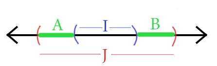
The two green intervals are our regions where error can occur.
If we can guarantee that each of the green pieces is smaller than $ \varepsilon / 2$ with high probability, then we’ll be done. Let’s look at $ A$, and the same argument will hold for $ B$. Define $ A’$ to be the interval $ [a_0, y]$ which is so big that the probability that a positive example is drawn from $ A’$ under $ D$ is exactly $ \varepsilon / 2$. Here’s another picture to clarify that.
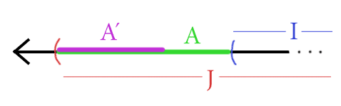
The pink region A' has total probability weight epsilon/2, and if the green region A is larger, we risk too much error to be PAC-learnable.
We’ll be in great shape if it’s already the case that $ A \subset A’$, because that implies the probability we draw a positive example from $ A$ is at most $ \varepsilon / 2$. So we’re worried about the possibility that $ A’ \subset A$. But this can only happen if we never saw a point from $ A’$ as a sample during the run of our algorithm. Since we had $ m$ samples, we can compute in terms of $ m$ the probability of never seeing a sample from $ A’$.
The probability of a single sample not being in $ A’$ is just $ 1 – \varepsilon/2$ (by definition!). Recalling our basic probability theory, two draws are independent events, and so the probability of missing $ A’$ $ m$ times is equal to the product of the probabilities of each individual miss. That is, the probability that our chosen $ A$ contributes error greater than $ \varepsilon / 2$ is at most
$$\displaystyle \textup{P}_D(A’ \subset A) \leq (1 – \varepsilon / 2)^m$$The same argument applies to $ B$, so we know by the union bound that the probability of error $ > \varepsilon / 2$ occurring in either $ A$ or $ B$ is at most the sum of the probabilities of large error in each piece, so that
$$\displaystyle \textup{P}_D(\textup{err}_{J,D}(I) > \varepsilon) \leq 2(1 – \varepsilon / 2)^m$$Now for the third bullet. We want the chance that the error is big to be smaller than $ \delta$, so that we’ll have low error with probability $ > 1 – \delta$. So simply set
$$\displaystyle 2(1 – \varepsilon / 2)^m \leq \delta$$And solve for $ m$. Using the fact that $ (1-x) \leq e^{-x}$ (which is proved by Taylor series), it’s enough to solve
$ \displaystyle 2e^{-\varepsilon m/2} \leq \delta$,
And a fine solution is $ m \geq (2 / \varepsilon \log (2 / \delta))$.
Now to cover all our bases: our algorithm simply computes $ m$ for its inputs $ \varepsilon, \delta$, queries that many samples, and computes the tightest-fitting interval containing the positive examples. Since the number of samples is polynomial in $ 1/\varepsilon, 1/\delta$ (and our algorithm doesn’t do anything complicated), we comply with the time and space bounds. And finally we just proved that the chance our algorithm will misclassify an $ \varepsilon$ fraction of new points drawn from $ D$ is at most $ \delta$. So we have proved the theorem:
Theorem: Intervals on the real line are PAC-learnable.
$$\square$$As an exercise, see if you can generalize the argument to axis-aligned rectangles in the plane. What about to arbitrary axis-aligned boxes in $ d$ dimensional space? Where does $ d$ show up in the number of samples needed? Is this still efficient?
Comments and Previews
There are a few more technical details we’ve ignored in the course of this post, but the important idea are clear. We have a formal model of learning which allows for certain pre-specified levels of imperfection, and we proved that one can learn how to recognize intervals in this model. It’s a far cry from decision trees and neural networks, but it’s a solid foundation to build upon.
However, the definition we presented here for PAC-learning is not quite complete. It turns out, as we’ll see in the next post, that forcing the PAC-learning algorithm to produce hypotheses from the same concept class it’s trying to learn makes some problems that should be easy hard. This is just because it could require the algorithm to represent some simple hypothesis in a convoluted form, and in the next post we’ll see that this is not an idle threat, and we’ll make a slight modification to the PAC definition.
However PAC-learning is far from sacred. In particular, the choice that we require a single algorithm to succeed no matter what the distribution $ D$ was a deliberate choice, and it’s quite a strong requirement for a learning algorithm. There are also versions of PAC that remove other assumptions from the definition, such that the oracle for the target concept is honest (noise-free) and that there is any available hypothesis that is actually true (realizability). These all give rise to interesting learning models and discovering the relationship between the models is the end goal.
And so the kinds of questions we ask are: can we classify all PAC-learnable problems? Can we find a meta-algorithm that would work on any PAC-learnable concept class given some assumptions? How does PAC-learning relate to other definitions of learning? Say, one where we don’t require it to work for every distribution; would that really allow us to solve more problems?
It’s a question of finding out the deep truths of mathematics now, but we promise that this series will soon come back around to practical applications, for learning theory naturally entails the design and analysis of fascinating algorithms.
Until next time!
Want to respond? Send me an email, post a webmention, or find me elsewhere on the internet.