A professor at Stanford once said,
If you really want to impress your friends and confound your enemies, you can invoke tensor products… People run in terror from the $ \otimes$ symbol.
He was explaining some aspects of multidimensional Fourier transforms, but this comment is only half in jest; people get confused by tensor products. It’s often for good reason. People who really understand tensors feel obligated to explain it using abstract language (specifically, universal properties). And the people who explain it in elementary terms don’t really understand tensors.
This post is an attempt to bridge the gap between the elementary and advanced understandings of tensors. We’ll start with the elementary (axiomatic) approach, just to get a good feel for the objects we’re working with and their essential properties. Then we’ll transition to the “universal” mode of thought, with the express purpose of enlightening us as to why the properties are both necessary and natural.
But above all, we intend to be sufficiently friendly so as to not make anybody run in fear. This means lots of examples and preferring words over symbols. Unfortunately, we simply can’t get by without the reader knowing the very basics of linear algebra (the content of our first two primers on linear algebra (1) (2), though the only important part of the second is the definition of an inner product).
So let’s begin.
Tensors as a Bunch of Axioms
Before we get into the thick of things I should clarify some basic terminology. Tensors are just vectors in a special vector space. We’ll see that such a vector space comes about by combining two smaller vector spaces via a tensor product. So the tensor product is an operation combining vector spaces, and tensors are the elements of the resulting vector space.
Now the use of the word product is quite suggestive, and it may lead one to think that a tensor product is similar or related to the usual direct product of vector spaces. In fact they are related (in very precise sense), but they are far from similar. If you were pressed, however, you could start with the direct product of two vector spaces and take a mathematical machete to it until it’s so disfigured that you have to give it a new name (the tensor product).
With that image in mind let’s see how that is done. For the sake of generality we’ll talk about two arbitrary finite-dimensional vector spaces $ V, W$ of dimensions $ n, m$. Recall that the direct product $ V \times W$ is the vector space of pairs $ (v,w)$ where $ v$ comes from $ V$ and $ w$ from $ W$. Recall that addition in this vector space is defined componentwise ($ (v_1,w_1) + (v_2, w_2) = (v_1 + v_2, w_1 + w_2$)) and scalar multiplication scales both components $ \lambda (v,w) = (\lambda v, \lambda w)$.
To get the tensor product space $ V \otimes W$, we make the following modifications. First, we redefine what it means to do scalar multiplication. In this brave new tensor world, scalar multiplication of the whole vector-pair is declared to be the same as scalar multiplication of any component you want. In symbols,
$$\displaystyle \lambda (v, w) = (\lambda v, w) = (v, \lambda w)$$for all choices of scalars $ \lambda$ and vectors $ v, w$. Second, we change the addition operation so that it only works if one of the two components are the same. In symbols, we declare that
$$(v, w) + (v’, w) = (v + v’, w)$$only works because $ w$ is the same in both pieces, and with the same rule applying if we switch the positions of $ v,w$ above. All other additions are simply declared to be new vectors. I.e. $ (x,y) + (z,w)$ is simply itself. It’s a valid addition — we need to be able to add stuff to be a vector space — but you just can’t combine it any further unless you can use the scalar multiplication to factor out some things so that $ y=w$ or $ x=z$. To say it still one more time, a general element of the tensor $ V \otimes W$ is a sum of these pairs that can or can’t be combined by addition (in general things can’t always be combined).
Finally, we rename the pair $ (v,w)$ to $ v \otimes w$, to distinguish it from the old vector space $ V \times W$ that we’ve totally butchered and reanimated, and we call the tensor product space as a whole $ V \otimes W$. Those familiar with this kind of abstract algebra will recognize quotient spaces at work here, but we won’t use that language except to note that we cover quotients and free spaces elsewhere on this blog, and that’s the formality we’re ignoring.
As an example, say we’re taking the tensor product of two copies of $ \mathbb{R}$. This means that our space $ \mathbb{R} \otimes \mathbb{R}$ is comprised of vectors like $ 3 \otimes 5$, and moreover that the following operations are completely legitimate.
$$3 \otimes 5 + 1 \otimes (-5) = 3 \otimes 5 + (-1) \otimes 5 = 2 \otimes 5$$ $$6 \otimes 1 + 3\pi \otimes \pi = 3 \otimes 2 + 3 \otimes \pi^2 = 3 \otimes (2 + \pi^2)$$Cool. This seemingly innocuous change clearly has huge implications on the structure of the space. We’ll get to specifics about how different tensors are from regular products later in this post, but for now we haven’t even proved this thing is a vector space. It might not be obvious, but if you go and do the formalities and write the thing as a quotient of a free vector space (as we mentioned we wouldn’t do) then you know that quotients of vector spaces are again vector spaces. So we get that one for free. But even without that it should be pretty obvious: we’re essentially just declaring that all the axioms of a vector space hold when we want them to. So if you were wondering whether
$$\lambda (a \otimes b + c \otimes d) = \lambda(a \otimes b) + \lambda(c \otimes d)$$The answer is yes, by force of will.
So just to recall, the axioms of a tensor space $ V \otimes W$ are
- The “basic” vectors are $ v \otimes w$ for $ v \in V, w \in W$, and they’re used to build up all other vectors.
- Addition is symbolic, unless one of the components is the same in both addends, in which case $ (v_1, w) + (v_2, w) = (v_1+ v_2, w)$ and $ (v, w_1) + (v,w_2) = (v, w_1 + w_2)$.
- You can freely move scalar multiples around the components of $ v \otimes w$.
- The rest of the vector space axioms (distributivity, additive inverses, etc) are assumed with extreme prejudice.
Naturally, one can extend this definition to $ n$-fold tensor products, like $ V_1 \otimes V_2 \otimes \dots \otimes V_d$. Here we write the vectors as sums of things like $ v_1 \otimes \dots \otimes v_d$, and we enforce that addition can only be combined if all but one coordinates are the same in the addends, and scalar multiples move around to all coordinates equally freely.
So where does it come from?!
By now we have this definition and we can play with tensors, but any sane mathematically minded person would protest, “What the hell would cause anyone to come up with such a definition? I thought mathematics was supposed to be elegant!”
It’s an understandable position, but let me now try to convince you that tensor products are very natural. The main intrinsic motivation for the rest of this section will be this:
We have all these interesting mathematical objects, but over the years we have discovered that the maps between objects are the truly interesting things.
A fair warning: although we’ll maintain a gradual pace and informal language in what follows, by the end of this section you’ll be reading more or less mature 20th-century mathematics. It’s quite alright to stop with the elementary understanding (and skip to the last section for some cool notes about computing), but we trust that the intrepid readers will push on.
So with that understanding we turn to multilinear maps. Of course, the first substantive thing we study in linear algebra is the notion of a linear map between vector spaces. That is, a map $ f: V \to W$ that factors through addition and scalar multiplication (i.e. $ f(v + v’) = f(v) + f(v’)$ and $ f(\lambda v) = \lambda f(v)$).
But it turns out that lots of maps we work with have much stronger properties worth studying. For example, if we think of matrix multiplication as an operation, call it $ m$, then $ m$ takes in two matrices and spits out their product
$$m(A,B) = AB$$Now what would be an appropriate notion of linearity for this map? Certainly it is linear in the first coordinate, because if we fix $ B$ then
$$m(A+C, B) = (A+C)B = AB + CB = m(A,B) + m(C,B)$$And for the same reason it’s linear in the second coordinate. But it is most definitely not linear in both coordinates simultaneously. In other words,
$$m(A+B, C+D) = (A+B)(C+D) = AC + AD + BC + BD \neq AC + BD = m(A,C) + m(B,D)$$In fact, there is only one function that satisfies both “linearity in its two coordinates separately” and also “linearity in both coordinates simultaneously,” and it’s the zero map! (Try to prove this as an exercise.) So the strongest kind of linearity we could reasonably impose is that $ m$ is linear in each coordinate when all else is fixed. Note that this property allows us to shift around scalar multiples, too. For example,
$$\displaystyle m(\lambda A, B) = \lambda AB = A (\lambda B) = m(A, \lambda B) = \lambda m(A,B)$$Starting to see the wispy strands of a connection to tensors? Good, but hold it in for a bit longer. This single-coordinate-wise-linear property is called bilinearity when we only have two coordinates, and multilinearity when we have more.
Here are some examples of nice multilinear maps that show up everywhere:
- If $ V$ is an inner product space over $ \mathbb{R}$, then the inner product is bilinear.
- The determinant of a matrix is a multilinear map if we view the columns of the matrix as vector arguments.
- The cross product of vectors in $ \mathbb{R}^3$ is bilinear.
There are many other examples, but you should have at least passing familiarity with these notions, and it’s enough to convince us that multilinearity is worth studying abstractly.
And so what tensors do is give a sort of classification of multilinear maps. The idea is that every multilinear map $ f$ from a product vector space $ U_1 \times \dots \times U_d$ to any vector space $ Y$ can be written first as a multilinear map to the tensor space
$$\displaystyle \alpha : U_1 \times \dots \times U_d \to U_1 \otimes \dots \otimes U_d$$Followed by a linear map to $ Y$,
$$\displaystyle \hat{f} : U_1 \otimes \dots \otimes U_d \to Y$$And the important part is that $ \alpha$ doesn’t depend on the original $ f$ (but $ \hat{f}$ does). One usually draws this as a single diagram:
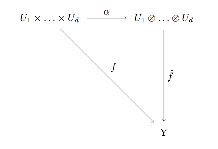
comm-diagram-tensor
And to say this diagram commutes is to say that all possible ways to get from one point to another are equivalent (the compositions of the corresponding maps you follow are equal, i.e. $ f = \hat{f} \alpha$).
In fuzzy words, the tensor product is like the gatekeeper of all multilinear maps, and $ \alpha$ is the gate. Yet another way to say this is that $ \alpha$ is the most general possible multilinear map that can be constructed from $ U_1 \times \dots \times U_d$. Moreover, the tensor product itself is uniquely defined by having a “most-general” $ \alpha$ (up to isomorphism). This notion is often referred to by mathematicians as the “universal property” of the tensor product. And they might say something like “the tensor product is initial with respect to multilinear mappings from the standard product.” We discuss language like this in detail in this blog’s series on category theory, but it’s essentially a super-compact (and almost too vague) way of saying what the diagram says.
Let’s explore this definition when we specialize to a tensor of two vector spaces, and it will give us a good understanding of $ \alpha$ (which is really incredibly simple, but people like to muck it up with choices of coordinates and summations). So fix $ V, W$ as vector spaces and look at the diagram
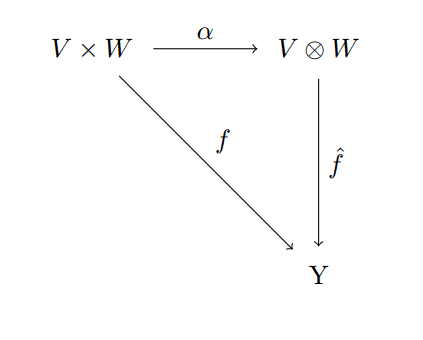
comm-diagram-tensor-2
What is $ \alpha$ in this case? Well it just sends $ (v,w) \mapsto v \otimes w$. Is this map multilinear? Well if we fix $ w$ then
$$\displaystyle \alpha(v_1 + v_2, w) = (v_1 + v_2) \otimes w = v_1 \otimes w + v_2 \otimes w = \alpha(v_1, w) + \alpha (v_2, w)$$and
$$\displaystyle \alpha(\lambda v, w) = (\lambda v) \otimes w = (\lambda) (v \otimes w) = \lambda \alpha(v,w)$$And our familiarity with tensors now tells us that the other side holds too. Actually, rather than say this is a result of our “familiarity with tensors,” the truth is that this is how we know that we need to define the properties of tensors as we did. It’s all because we designed tensors to be the gatekeepers of multilinear maps!
So now let’s prove that all maps $ f : V \times W \to Y$ can be decomposed into an $ \alpha$ part and a $ \hat{f}$ part. To do this we need to know what data uniquely defines a multilinear map. For usual linear maps, all we had to do was define the effect of the map on each element of a basis (the rest was uniquely determined by the linearity property). We know what a basis of $ V \times W$ is, it’s just the union of the bases of the pieces. Say that $ V$ has a basis $ v_1, \dots, v_n$ and $ W$ has $ w_1, \dots, w_m$, then a basis for the product is just $ ((v_1, 0), \dots, (v_n,0), (0,w_1), \dots, (0,w_m))$.
But multilinear maps are more nuanced, because they have two arguments. In order to say “what they do on a basis” we really need to know how they act on all possible pairs of basis elements. For how else could we determine $ f(v_1 + v_2, w_1)$? If there are $ n$ of the $ v_i$’s and $ m$ of the $ w_i$’s, then there are $ nm$ such pairs $ f(v_i, w_j)$.
Uncoincidentally, as $ V \otimes W$ is a vector space, its basis can also be constructed in terms of the bases of $ V$ and $ W$. You simply take all possible tensors $ v_i \otimes w_j$. Since every $ v \in V, w \in W$ can be written in terms of their bases, it’s clear than any tensor $ \sum_{k} a_k \otimes b_k$ can also be written in terms of the basis tensors $ v_i \otimes w_j$ (by simply expanding each $ a_k, b_k$ in terms of their respective bases, and getting a larger sum of more basic tensors).
Just to drive this point home, if $ (e_1, e_2, e_3)$ is a basis for $ \mathbb{R}^3$, and $ (g_1, g_2)$ a basis for $ \mathbb{R}^2$, then the tensor space $ \mathbb{R}^3 \otimes \mathbb{R}^2$ has basis
$$(e_1 \otimes g_1, e_1 \otimes g_2, e_2 \otimes g_1, e_2 \otimes g_2, e_3 \otimes g_1, e_3 \otimes g_2)$$It’s a theorem that finite-dimensional vector spaces of equal dimension are isomorphic, so the length of this basis (6) tells us that $ \mathbb{R}^3 \otimes \mathbb{R}^2 \cong \mathbb{R}^6$.
So fine, back to decomposing $ f$. All we have left to do is use the data given by $ f$ (the effect on pairs of basis elements) to define $ \hat{f} : V \otimes W \to Y$. The definition is rather straightforward, as we have already made the suggestive move of showing that the basis for the tensor space ($ v_i \otimes w_j$) and the definition of $ f(v_i, w_j)$ are essentially the same.
That is, just take $ \hat{f}(v_i \otimes w_j) = f(v_i, w_j)$. Note that this is just defined on the basis elements, and so we extend to all other vectors in the tensor space by imposing linearity (defining $ \hat{f}$ to split across sums of tensors as needed). Is this well defined? Well, multilinearity of $ f$ forces it to be so. For if we had two equal tensors, say, $ \lambda v \otimes w = v \otimes \lambda w$, then we know that $ f$ has to respect their equality, because $ f(\lambda v_i, w_j) = f(v_i, \lambda w_j)$, so $ \hat{f}$ will take the same value on equal tensors regardless of which representative we pick (where we decide to put the $ \lambda$). The same idea works for sums, so everything checks out, and $ f(v,w)$ is equal to $ \hat{f} \alpha$, as desired. Moreover, we didn’t make any choices in constructing $ \hat{f}$. If you retrace our steps in the argument, you’ll see that everything was essentially decided for us once we fixed a choice of a basis (by our wise decisions in defining $ V \otimes W$). Since the construction would be isomorphic if we changed the basis, our choice of $ \hat{f}$ is unique.
There is a lot more to say about tensors, and indeed there are some other useful ways to think about tensors that we’ve completely ignored. But this discussion should make it clear why we define tensors the way we do. Hopefully it eliminates most of the mystery in tensors, although there is still a lot of mystery in trying to compute stuff using tensors. So we’ll wrap up this post with a short discussion about that.
Computability and Stuff
It should be clear by now that plain product spaces $ V \times W$ and tensor product spaces $ V \otimes W$ are extremely different. In fact, they’re only related in that their underlying sets of vectors are built from pairs of vectors in $ V$ and $ W$. Avid readers of this blog will also know that operations involving matrices (like row reduction, eigenvalue computations, etc.) are generally efficient, or at least they run in polynomial time so they’re not crazy impractically slow for modest inputs.
On the other hand, it turns out that almost every question you might want to ask about tensors is difficult to answer computationally. As with the definition of the tensor product, this is no mere coincidence. There is something deep going on with tensors, and it has serious implications regarding quantum computing. More on that in a future post, but for now let’s just focus on one hard problem to answer for tensors.
As you know, the most general way to write an element of a tensor space $ U_1 \otimes \dots \otimes U_d$ is as a sum of the basic-looking tensors.
$$\sum_k \displaystyle a_{1,k} \otimes a_{2,k} \otimes \dots \otimes a_{d,k}$$where the $ a_{i,d}$ are linear combinations of basis vectors in the $ U_i$. But as we saw with our examples over $ \mathbb{R}$, there can be lots of different ways to write a tensor. If you’re lucky, you can write the entire tensor as a one-term sum, that is just a tensor $ a_1 \otimes \dots \otimes a_d$. If you can do this we call the tensor a pure tensor, or a rank 1 tensor. We then have the following natural definition and problem:
Definition: The rank of a tensor $ x \in U_1 \otimes \dots \otimes U_d$ is the minimum number of terms in any representation of $ x$ as a sum of pure tensors. The one exception is the zero element, which has rank zero by convention.
Problem: Given a tensor $ x \in k^{n_1} \otimes k^{n_2} \otimes k^{n_3}$ where $ k$ is a field, compute its rank.
Of course this isn’t possible in standard computing models unless you can represent the elements of the field (and hence the elements of the vector space in question) in a computer program. So we restrict $ k$ to be either the rational numbers $ \mathbb{Q}$ or a finite field $ \mathbb{F}_{q}$.
Even though the problem is simple to state, it was proved in 1990 (a result of Johan Håstad) that tensor rank is hard to compute. Specifically, the theorem is that
Theorem: Computing tensor rank is NP-hard when $ k = \mathbb{Q}$ and NP-complete when $ k$ is a finite field.
The details are given in Håstad’s paper, but the important work that followed essentially showed that most problems involving tensors are hard to compute (many of them by reduction from computing rank). This is unfortunate, but also displays the power of tensors. In fact, tensors are so powerful that many believe understanding them better will lead to insight in some very important problems, like finding faster matrix multiplication algorithms or proving circuit lower bounds (which is closely related to P vs NP). Finding low-rank tensor approximations is also a key technique in a lot of recent machine learning and data mining algorithms.
With this in mind, the enterprising reader will probably agree that understanding tensors is both valuable and useful. In the future of this blog we’ll hope to see some of these techniques, but at the very least we’ll see the return of tensors when we delve into quantum computing.
Until next time!