Fixing Bugs in "Computing Homology"

A few awesome readers have posted comments in Computing Homology to the effect of, “Your code is not quite correct!” And they’re right! Despite the almost year since that post’s publication, I haven’t bothered to test it for more complicated simplicial complexes, or even the basic edge cases! When I posted it the mathematics just felt so solid to me that it had to be right (the irony is rich, I know).

As such I’m apologizing for my lack of rigor and explaining what went wrong, the fix, and giving some test cases. As of the publishing of this post, the Github repository for Computing Homology has been updated with the correct code, and some more examples.

The main subroutine was the simultaneousReduce function which I’ll post in its incorrectness below

def simultaneousReduce(A, B):
   if A.shape[1] != B.shape[0]:
      raise Exception("Matrices have the wrong shape.")

   numRows, numCols = A.shape # col reduce A

   i,j = 0,0
   while True:
      if i >= numRows or j >= numCols:
         break

      if A[i][j] == 0:
         nonzeroCol = j
         while nonzeroCol < numCols and A[i,nonzeroCol] == 0:
            nonzeroCol += 1

         if nonzeroCol == numCols:
            j += 1
            continue

         colSwap(A, j, nonzeroCol)
         rowSwap(B, j, nonzeroCol)

      pivot = A[i,j]
      scaleCol(A, j, 1.0 / pivot)
      scaleRow(B, j, 1.0 / pivot)

      for otherCol in range(0, numCols):
         if otherCol == j:
            continue
         if A[i, otherCol] != 0:
            scaleAmt = -A[i, otherCol]
            colCombine(A, otherCol, j, scaleAmt)
            rowCombine(B, j, otherCol, -scaleAmt)

      i += 1; j+= 1

   return A,B

It’s a beast of a function, and the persnickety detail was just as beastly: this snippet should have an $ i += 1$ instead of a $ j$.

if nonzeroCol == numCols:
   j += 1
   continue

This is simply what happens when we’re looking for a nonzero entry in a row to use as a pivot for the corresponding column, but we can’t find one and have to move to the next row. A stupid error on my part that would be easily caught by proper test cases.

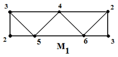
The next mistake is a mathematical misunderstanding. In short, the simultaneous column/row reduction process is not enough to get the $ \partial_{k+1}$ matrix into the right form! Let’s see this with a nice example, a triangulation of the Mobius band. There are a number of triangulations we could use, many of which are seen in these slides. The one we’ll use is the following.

It’s first and second boundary maps are as follows (in code, because latex takes too much time to type out)

mobiusD1 = numpy.array([
   [-1,-1,-1,-1, 0, 0, 0, 0, 0, 0],
   [ 1, 0, 0, 0,-1,-1,-1, 0, 0, 0],
   [ 0, 1, 0, 0, 1, 0, 0,-1,-1, 0],
   [ 0, 0, 0, 1, 0, 0, 1, 0, 1, 1],
])

mobiusD2 = numpy.array([
   [ 1, 0, 0, 0, 1],
   [ 0, 0, 0, 1, 0],
   [-1, 0, 0, 0, 0],
   [ 0, 0, 0,-1,-1],
   [ 0, 1, 0, 0, 0],
   [ 1,-1, 0, 0, 0],
   [ 0, 0, 0, 0, 1],
   [ 0, 1, 1, 0, 0],
   [ 0, 0,-1, 1, 0],
   [ 0, 0, 1, 0, 0],
])

And if we were to run the above code on it we’d get a first Betti number of zero (which is incorrect, it’s first homology group has rank 1). Here are the reduced matrices.

>>> A1, B1 = simultaneousReduce(mobiusD1, mobiusD2)
>>> A1
array([[1, 0, 0, 0, 0, 0, 0, 0, 0, 0],
       [0, 1, 0, 0, 0, 0, 0, 0, 0, 0],
       [0, 0, 1, 0, 0, 0, 0, 0, 0, 0],
       [0, 0, 0, 1, 0, 0, 0, 0, 0, 0]])
>>> B1
array([[ 0,  0,  0,  0,  0],
       [ 0,  0,  0,  0,  0],
       [ 0,  0,  0,  0,  0],
       [ 0,  0,  0,  0,  0],
       [ 0,  1,  0,  0,  0],
       [ 1, -1,  0,  0,  0],
       [ 0,  0,  0,  0,  1],
       [ 0,  1,  1,  0,  0],
       [ 0,  0, -1,  1,  0],
       [ 0,  0,  1,  0,  0]])

The first reduced matrix looks fine; there’s nothing we can do to improve it. But the second one is not quite fully reduced! Notice that rows 5, 8 and 10 are not linearly independent. So we need to further row-reduce the nonzero part of this matrix before we can read off the true rank in the way we described last time. This isn’t so hard (we just need to reuse the old row-reduce function we’ve been using), but why is this allowed? It’s just because the corresponding column operations for those row operations are operating on columns of all zeros! So we need not worry about screwing up the work we did in column reducing the first matrix, as long as we only work with the nonzero rows of the second.

Of course, nothing is stopping us from ignoring the “corresponding” column operations, since we know we’re already done there. So we just have to finish row reducing this matrix.

This changes our bettiNumber function by adding a single call to a row-reduce function which we name so as to be clear what’s happening. The resulting function is

def bettiNumber(d_k, d_kplus1):
   A, B = numpy.copy(d_k), numpy.copy(d_kplus1)
   simultaneousReduce(A, B)
   finishRowReducing(B)

   dimKChains = A.shape[1]
   kernelDim = dimKChains - numPivotCols(A)
   imageDim = numPivotRows(B)

   return kernelDim - imageDim

And running this on our Mobius band example gives:

>>> bettiNumber(mobiusD1, mobiusD2))
1

As desired. Just to make sure things are going swimmingly under the hood, we can check to see how finishRowReducing does after calling simultaneousReduce

>>> simultaneousReduce(mobiusD1, mobiusD2)
(array([[1, 0, 0, 0, 0, 0, 0, 0, 0, 0],
       [0, 1, 0, 0, 0, 0, 0, 0, 0, 0],
       [0, 0, 1, 0, 0, 0, 0, 0, 0, 0],
       [0, 0, 0, 1, 0, 0, 0, 0, 0, 0]]), array([[ 0,  0,  0,  0,  0],
       [ 0,  0,  0,  0,  0],
       [ 0,  0,  0,  0,  0],
       [ 0,  0,  0,  0,  0],
       [ 0,  1,  0,  0,  0],
       [ 1, -1,  0,  0,  0],
       [ 0,  0,  0,  0,  1],
       [ 0,  1,  1,  0,  0],
       [ 0,  0, -1,  1,  0],
       [ 0,  0,  1,  0,  0]]))
>>> finishRowReducing(mobiusD2)
array([[1, 0, 0, 0, 0],
       [0, 1, 0, 0, 0],
       [0, 0, 1, 0, 0],
       [0, 0, 0, 1, 0],
       [0, 0, 0, 0, 1],
       [0, 0, 0, 0, 0],
       [0, 0, 0, 0, 0],
       [0, 0, 0, 0, 0],
       [0, 0, 0, 0, 0],
       [0, 0, 0, 0, 0]])

Indeed, finishRowReducing finishes row reducing the second boundary matrix. Note that it doesn’t preserve how the rows of zeros lined up with the pivot columns of the reduced version of $ \partial_1$ as it did in the previous post, but since in the end we’re only counting pivots it doesn’t matter how we switch rows. The “zeros lining up” part is just for a conceptual understanding of how the image lines up with the kernel for a valid simplicial complex.

In fixing this issue we’ve also fixed an issue another commenter mentioned, that you couldn’t blindly plug in the zero matrix for $ \partial_0$ and get zeroth homology (which is the same thing as connected components). After our fix you can.

Of course there still might be bugs, but I have so many drafts lined up on this blog (and research papers to write, experiments to run, theorems to prove), that I’m going to put off writing a full test suite. I’ll just have to update this post with new bug fixes as they come. There’s just so much math and so little time 🙂 But extra kudos to my amazing readers who were diligent enough to run examples and spot my error. I’m truly blessed to have you on my side.

Also note that this isn’t the most efficient way to represent the simplicial complex data, or the most efficient row reduction algorithm. If you’re going to run the code on big inputs, I suggest you take advantage of sparse matrix algorithms for doing this sort of stuff. You can represent the simplices as entries in a dictionary and do all sorts of clever optimizations to make the algorithm effectively linear time in the number of simplices.

Until next time!