Last time we looked at the elementary formulation of an elliptic curve as the solutions to the equation
$$y^2 = x^3 + ax + b$$where $ a,b$ are such that the discriminant is nonzero:
$$-16(4a^3 + 27b^2) \neq 0$$We have yet to explain why we want our equation in this form, and we will get to that, but first we want to take our idea of intersecting lines as far as possible.
Fair warning: this post will start out at the same level as the previous post, but we intend to gradually introduce some mathematical maturity. If you don’t study mathematics, you’ll probably see terminology and notation somewhere between mysterious and incomprehensible. In particular, we will spend a large portion of this post explaining projective coordinates, and we use the blackboard-bold $ \mathbb{R}$ to denote real numbers.
Skimming difficult parts, asking questions in the comments, and pushing through to the end are all encouraged.
The Algorithm to Add Points
The deep idea, and the necessary insight for cryptography, is that the points on an elliptic curve have an algebraic structure. What I mean by this is that you can “add” points in a certain way, and it will satisfy all of the properties we expect of addition with true numbers. You may have guessed it based on our discussion in the previous post: adding two points will involve taking the line passing between them and finding the third point of intersection with the elliptic curve. But in order to make “adding points” rigorous we need to deal with some special cases (such as the vertical line problem we had last time).
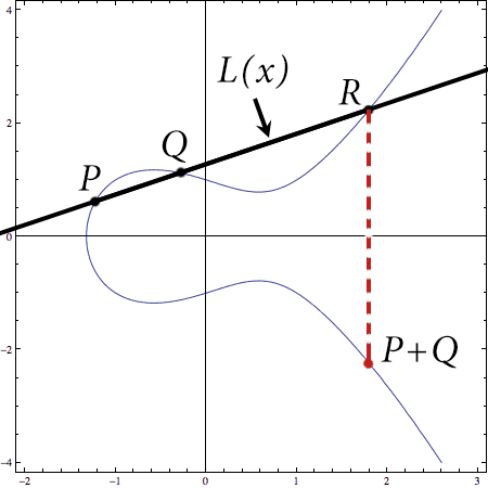
So say we have two points $ P, Q$ on an elliptic curve $ E$ defined by $ y^2 = x^3 + ax + b$. By saying they’re “on the curve” we mean their coordinates satisfy the equation defining the curve. Then to add $ P + Q$, we do the following geometric algorithm:
- Form the line $ y = L(x)$ connecting $ P$ and $ Q$.
- Compute the third intersection point of $ L$ with $ E$ (the one that’s not $ P$ or $ Q$). Call it $ R$.
- Reflect $ R$ across the $ x$-axis to get the final point $ P + Q$.
Here’s that shown visually on our practice curve $ E: y^2 = x^3 – x + 1$.
add-points-example
This algorithm might seem dubious, but it’s backed up by solid mathematics. For example, it’s almost immediately obvious that step 1 will always work (that you can always form such a line), the only exception being when $ P = Q$. And it’s almost a theorem that step 2 will always work (that there is always a third point of intersection), the only exception being the vertical line. If we ignore these exceptional cases, then the correctness of the algorithm is easy to prove, because we can just generalize the idea from last time.
Solving the joint system of the curve and the line is equivalent to solving
$$L(x)^2 = x^3 + ax + b$$Since $ L(x)$ is a degree 1 polynomial, this equation is a cubic polynomial in $ x$
$$x^3 – L(x)^2 + ax + b = 0$$If we already have two solutions to this equation with distinct $ x$-values (two points on the curve that don’t form a vertical line) then there has to be a third. Why? Because having a root of a polynomial means you can factor, and we have two distinct roots, so we know that our polynomial has as a divisor
$$(x – p_1)(x – q_1)$$But then the remainder must be a linear polynomial, and because the leading term is $ x^3$ it has to look like $ (x – r_1)$ for some $ r_1$. And so $ (r_1, L(r_1))$ is our third point. Moreover, $ p_1 + r_1 + q_1$ must be equal to the opposite of the coefficient of $ x^2$ in the equation above, so we can solve for it without worry about how to factor cubic polynomials. When we get down to some nitty-gritty code we’ll need to be more precise here with equations and such, but for now this is good enough.
Pause, Breathe, Reflect
It’s time to take a step back. There is a big picture overarching our work here. We have this mathematical object, a bunch of points on a curve in space, and we’re trying to say that it has algebraic structure. As we’ve been saying, we want to add points on the curve using our algorithm and always get a point on the curve as a result.
But beyond the algorithm, two important ideas are at work here. The first is that any time you make a new mathematical definition with the intent of overloading some operators (in this case, + and -), you want to make sure the operators behave like we expect them to. Otherwise “add” is a really misleading name!
The second idea is that we’re encoding computational structure in an elliptic curve. The ability to add and negate opens up a world of computational possibilities, and so any time we find algebraic structure in a mathematical object we can ask questions about the efficiency of computing functions within that framework (and reversing them!). This is precisely what cryptographers look for in a new encryption scheme: functions which are efficient to compute, but very hard to reverse if all you know is the output of the function.
So what are the properties we need to make sure addition behaves properly?
- We need there to be an the additive identity, which we’ll call zero, for which $ P + 0 = 0 + P = P$.
- We need every point $ P$ to have an inverse $ -P$ for which $ P + (-P) = 0$.
- We want adding to commute, so that $ P + Q = Q + P$. This property of an algebraic structure is called abelian or commutative.
- We need addition to be associative, so that $ (P + Q) + R = P + (Q + R)$.
In fact, if you just have a general collection of things (a set, in the mathematical parlance) and an operation which together satisfy these four properties, we call that a commutative group. By the end of this series we’ll to switch to the terminology of groups to get a mathematically mature viewpoint on elliptic curves, because it turns out that not all types of algebraic structure are the same (there are lots of different groups). But we’ll introduce it slowly as we see why elliptic curves form groups under the addition of their points.
There are still some things about our adding algorithm above that aren’t quite complete. We still need to know:
- What will act as zero.
- How to get the additive inverse of a point.
- How to add a point to itself.
- What to do if the two points form a vertical line.
The first, second, and fourth items are all taken care of in one fell swoop (and this is the main bit of mathematical elbow grease we have been hinting at), but the third point has a quick explanation if you’re willing to postpone a technical theorem. If you want to double a point, or add $ P + P = 2P$, then you can’t “take the line joining those two points” because you need two distinct points to define a line. But you can take the tangent line to the curve at $ P$ and look for the second point of intersection. Again we still have to worry about the case of a vertical line. But ignoring that, the reason there will always be a second point of intersection is called Bezout’s theorem, and this theorem is so strong and abstract that it’s very difficult to discuss it with what we presently know, but it has to do with counting multiplicity of roots of polynomial equations. Seeing that it’s mostly a technical tool, we’ll just be glad it’s there.
So with that, let’s get to the most important bit.
Projective Space and the Ideal Line
The shortest way to describe what will act as zero in our elliptic curve is to say that we invent a new point which is the “intersection” of all vertical lines. Because it’s the intersection of vertical lines, we’ll sometimes call it “the point at infinity.” We’ll also call it “zero” because it’s supposed to be the additive identity, we’ll demand it lies on every elliptic curve, and we’ll enforce that if we “reflect” zero across the $ x$-axis we still get zero. And then everything works!
If you want to add two points that form a vertical line, well, now the third point of intersection is zero and reflecting zero still gives you zero. If you want to get the additive inverse of a point $ P = (x,y)$, just have it be the point $ -P = (x, -y)$ reflected across the $ x$-axis; the two points form a vertical line and so by our algorithm they “add up” to zero. So it’s neat and tidy.
But wait, wait, wait. Points at infinity? All vertical lines intersect? This isn’t like any geometry I’ve ever seen before. How do we know we can do this without getting some massive contradictions!?
This is the best question one could ask, and we refuse to ignore it. Many articles aimed at a general technically literate audience get very fuzzy at this part. They make it seem like the mathematics we’re doing is magic, and they ignore the largest mathematical elephant in the room. Of course it’s not magic, and all of this has a solid foundation called projective space. We’re going to explore its basics now.
There is a long history of arguing over Euclid’s geometric axioms and how the postulate that parallel lines never intersect doesn’t follow from the other axioms. This is exactly what we’re going for, but blah blah blah let’s just see the construction already!
The crazy brilliant idea is that we want to make a geometric space where points are actually lines.
What will happen is that our elliptic curve equations will get an extra variable to account for this new kind of geometry, and a special value for this new variable will allow us to recover the usual pictures of elliptic curves in the plane (this is intentionally vague and will become more precise soon).
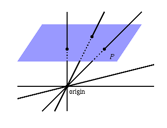
So how might one make such a geometry? Well you can do it with or without linear algebra. The way without linear algebra is to take three dimensional Euclidean space $ \mathbb{R}^3$, and look at the lines that pass through the origin. Make each of these lines its own point, and call the resulting space $ \mathbb{P}^2$, the projective plane. (For avid readers of this blog, this is exactly the same construction as $ \mathbb{R}\textup{P}^2$ we gave in our second topology primer, just seen from a very different angle. Leave a comment if you want to hear more.)
The problem with the non-linear-algebra approach is that we get no natural coordinate system, and we’re dying for coordinates (we’re here to compute stuff, after all!). So we need to talk about vectors. Every nonzero vector $ v$ in $ \mathbb{R}^3$ spans a line (by taking all multiples $ \lambda v$ for $ \lambda \in \mathbb{R}$). So instead of representing a point in projective space by a line, we can represent it by a vector, with the additional condition that two points are the same if they’re multiples of each other.
Here’s a picture of this idea. The two vectors displayed are equal to each other because they lie on the same line (they are multiples of each other).
These two vectors are equivalent because they lie on (span) the same line.
Don’t run away because a very detailed explanation will follow what I’m about to say, but the super formal way of saying this is that projective space is the quotient space
$$\displaystyle \mathbb{P}^2 = (\mathbb{R}^3 – \left \{ 0 \right \} ) / v \sim \lambda v$$Still here? Okay great. Let’s talk about coordinates. If we are working with vectors in $ \mathbb{R}^3$, then we’re looking at coordinates like
$$(x, y, z)$$where $ x,y,z$ are real numbers. Trivial. But now in projective space we’re asserting two things. First, $ (0,0,0)$ is not allowed. And second, whenever we have $ (x,y,z)$, we’re declaring that it’s the same thing as $ (2x,2y,2z)$ or $ (-6x, -6y, -6z)$ or any other way to scale every component by the same amount. To denote the difference between usual vectors (parentheses) and our new coordinates, we use square brackets and colons. So a point in 2-dimensional projective space is
$$[x:y:z]$$where $ x,y,z$ are real numbers that are not all zero, and $ [x:y:z] = \lambda [x : y : z] = [\lambda x : \lambda y : \lambda z]$ for any $ \lambda \in \mathbb{R}$.
Now we can make some “canonical choices” for our coordinates, and start exploring how the assertions we made shape the geometry of this new space. For example, if $ P = [x:y:z]$ with $ z \neq 0$ then we can always scale by $ 1/z$ so that the point looks like
$$[x/z : y/z : 1]$$Now $ x/z$ and $ y/z$ can be anything (just think of it as $ [a : b : 1]$), and different choices of $ a,b$ give distinct points. Why? Because if we tried to scale to make two points equal we’d be screwing up the 1 that’s fixed in the third coordinate. So when $ z$ is nonzero we have this special representation (often called an affine slice), and it’s easy to see that all of these points form a copy of the usual Euclidean plane sitting inside $ \mathbb{P}^2$. There is a nice way to visualize exactly how this copy can be realized as “usual Euclidean space” using the picture below:
proj-eucl-ex
Each line (each vector with $ z \neq 0$) intersects the indigo plane in exactly one point, so this describes a one-to-one mapping of points in the affine slice to the Euclidean plane.
But then when $ z = 0$, we get some other stuff that makes up the rest of $ \mathbb{P}^2$. Since $ x,y$ can’t both also be zero, we’ll suppose $ y$ is not zero, and then we can do the same normalization trick to see that all the points we get are
$$[a : 1 : 0]$$Since again $ a$ can be anything and you get distinct points for different choices of $ a$, this forms a copy of the real line inside of $ \mathbb{P}^2$ but outside of the affine slice. This line is sometimes called the ideal line to distinguish it from the lines that lie inside the affine slice $ z=1$. Actually, the ideal line is more than just a line. It’s (gasp) a circle! Why do I say that? Well think about what happens as $ a$ gets really large (or really negatively large). We have
$$[a : 1 : 0] = [1 : 1/a : 0]$$and the right hand side approaches $ [1 : 0 : 0]$, the last missing point! Another way to phrase our informal argument is to say $ [1 : 0 : 0]$ is the boundary of the line $ [a : 1 : 0]$, and (you guessed it) the circle we get here is the boundary of the affine slice $ [a : b : 1]$. And we can see exactly what it means for “two parallel lines” to intersect. Take the two lines given by
$$[a : 1 : 1], [b : 2 : 1]$$If we think of these as being in the affine slice of $ \mathbb{R}^2$ where $ z = 1$, it’s the lines given by $ (a, 1), (b, 2)$, which are obviously parallel. But where do they intersect as $ a,b$ get very large (or very negatively large)? at
$$[1 : 1/a : 1/a], [1 : 2/b : 1/b]$$which both become $ [1 : 0 : 0]$ in the limit. I’m being a bit imprecise here appealing to limits, but it works because projective space inherits some structure when we pass to the quotient (for the really technically inclined, it inherits a metric that comes from the sphere of radius 1). This is why we feel compelled to call it a quotient despite how confusing quotients can be, and it illustrates the power of appealing to these more abstract constructions.
In any case, now we have this image of projective space:
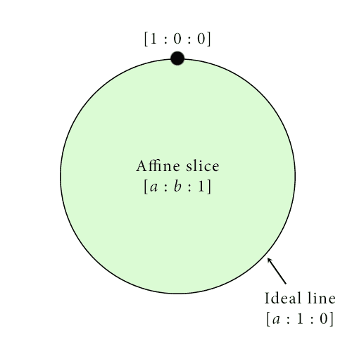
Our mental image of the projective plane: a big copy of the Euclidean plane (affine slice) whose boundary is the ideal line, whose boundary is in turn the single point [1:0:0].
It should be pretty clear that the choice of $ z=1$ to represent the affine slice is arbitrary, and we could have used $ x=1$ or $ y=1$ to realize different “copies” of the Euclidean plane sitting inside projective space. But in any case, we can use our new understanding to turn back to elliptic curves.
Homogeneous Equations and the Weierstrass Normal Form
Elliptic curves are officially “projective objects” in the sense that they are defined by homogeneous equations over projective space. That is, an elliptic curve equation is any homogeneous degree three equation whose discriminant is zero. By homogeneous I mean all the powers of the terms add up to three, so it has the general form
$$0 = a_0 z^3 + a_1 z^2y + a_2 z^2x + a_3y^2x + \dots$$And note that now the solutions to this equation are required to be projective points $ [x : y : z]$. As an illuminating exercise, prove that $ [x : y : z]$ is a solution if and only if $ [\lambda x : \lambda y: \lambda z]$ is, i.e. that our definition of “solution” and the use of homogeneous equations is well-defined.
But to work with projective language forever is burdensome, something that only mathematicians are required to do. And in the case of elliptic curves we only use one new point from projective space (the intersection of the vertical lines). Once we get to writing programs we’ll have a special representation for points that aren’t in the affine slice, so we will be able to use regular Euclidean coordinates without much of a fuss.
That being said, we can now officially explain why we want the special form of elliptic curve $ y^2 = x^3 + ax + b$, called the Weierstrass normal form (pronounced VY-er-shtrahss). Specifically, elliptic curves can look very weird in their natural coordinates.
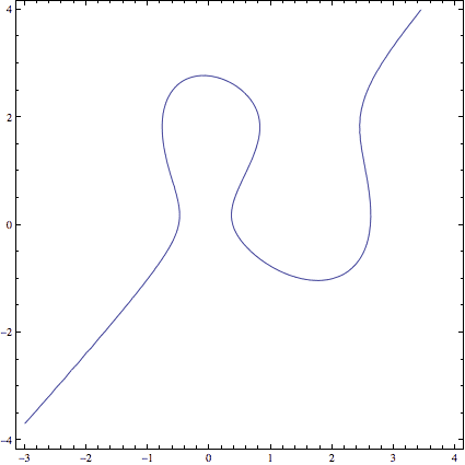
An elliptic curve before being converted to Weierstrass normal form.
So to bring some order to the chaos, we want the projective point $ [0 : 1 : 0]$ to be our zero point. If we choose our axes appropriately (swapping the letters $ x, y, z$), then $ [0:1:0]$ lies at the intersection of all vertical lines. Now that point isn’t a solution to all homogeneous degree-three curves, but it is a solution to homogeneous equations that look like this (plug it in to see).
$$\displaystyle y^2z = x^3 + ax z^2 + b z^3$$Starting to look familiar? It turns out there is a theorem (that requires either heavy mathematical machinery or LOTS of algebra to prove) that says that for any homogeneous degree three equation you start with, you can always pick your “projective axes” (that is, apply suitable projective transformations) to get an equivalent equation of the form above. I mean equivalent in the sense that the transformation we applied took solutions of the original equation to solutions of this new equation and didn’t create any new ones. The casual reader should think of all this machinery as really clever changes of variables.
And then if we pick our classical Euclidean slice to be $ [x : y : 1]$, we get back to the standard form $ y^2 = x^3 + ax + b$. This is the Weierstrass normal form.
So that was a huge detour…
Back to adding points on elliptic curves. Now that we’ve defined zero one can check that addition makes sense. Zero has the needed property $ P + 0 = P$ since the “third” point of intersection of the vertical line passing through $ P$ is the reflection of $ P$ across the $ x$-axis, and reflecting that across the $ x$-axis give you $ P$. For the same reason $ P + (-P) = 0$. Even more, properties like $ 0 = -0$ naturally fall out of our definitions for projective coordinates, since $ [0:1:0] = [0:-1:0] = -1[0:1:0]$. So projective space, rather than mathematical hocus-pocus, is the correct setting to think about algebra happening on elliptic curves.
It’s also clear that addition is commutative because lines passing through points don’t care about the order of the points. The only real issue is whether addition is associative. That is whether $ (P + Q) + R = P + (Q + R)$ no matter what $ P,Q,R$ are. This turns out to be difficult, and it takes a lot of algebra and the use of that abstract Bezout’s theorem we mentioned earlier, so the reader will have to trust us that everything works out. (Although, Wikipedia has a slick animation outlining one such proof.)
So “adding points,” and that pesky “point at infinity” now officially makes sense!
What we’ve shown in the mathematical parlance is that the solutions to an elliptic curve form a group under this notion of addition. However, one thing we haven’t talked about is where these numbers come from. Recall from last time that we were interested in integer points on the elliptic curve, but it was clear from our example that adding two integer-valued points on an elliptic curve might not give you an integer-valued point.
However, if we require that our equation has coefficients in a field, and we allow our points to have coordinates in that same field, then adding two points with coordinates in the field always gives you a point with coordinates in the field. We haven’t ever formally talked about fields on this blog, but we’re all familiar with them: they have addition, multiplication, and division in the expected ways (everything except 0 has a multiplicative inverse, multiplication distributes across addition, etc.). The usual examples are $ \mathbb{R}, \mathbb{C}$ the real and complex numbers, and $ \mathbb{Q}$, the rational numbers (fractions of integers). There are also finite fields, which are the proper setting for elliptic curve cryptography, but we’ll save those for another post.
But why must it work if we use a field? Because the operations we need to perform the point-adding algorithm only use field operations (addition, multiplication, and division by other numbers in the field). So performing those operations on numbers in a field always give you back numbers in that field. Since all fields have 0 and 1, we also have the point at infinity $ [0 : 1 : 0]$.
This gives a natural definition.
Definition: Let $ k$ be a field and let $ E$ be the equation of an elliptic curve in Weierstrass form. Define $ E(k)$ to be the set of projective points on $ E$ with coordinates in $ k$ along with the ideal point $ [0:1:0]$. As we have discussed $ E(k)$ is a group under the operation of adding points, so we call it the elliptic curve group for $ E$ over $ k$.
Now that we’ve waded through a few hundred years of mathematics, it should be no surprise that this definition feels so deep and packed full of implicit understanding.
However, there are still a few mathematical peccadilloes to worry about. One is that if the chosen field $ k$ is particularly weird (as are many of those finite fields I mentioned), then we can’t transform any equation with coefficients in $ k$ into the Weierstrass normal form. This results in a few hiccups when you’re trying to do cryptography, but for simplicity’s sake we’ll avoid those areas and stick to nicer fields.
We have only scratched the surface of the algebraic structure of elliptic curves by showing elliptic curves have such structure at all. The next goal for a mathematician is to classify all possible algebraic structures for elliptic curves , and find easy ways to tell which from the coefficients of the equation. Indeed, we intend to provide a post at the end of this series (after we get to the juicy programs) that describes what’s known in this area from a more group-theoretic standpoint (i.e., for someone who has heard of the classification of finitely generated abelian groups).
But before that we’re ready to jump headfirst into some code. Next time we’ll implement the algorithms for adding points on elliptic curves using Python objects.
Until then!
Want to respond? Send me an email, post a webmention, or find me elsewhere on the internet.