A problem that is not (properly) PAC-learnable

In a previous post we introduced a learning model called Probably Approximately Correct (PAC). We saw an example of a concept class that was easy to learn: intervals on the real line (and more generally, if you did the exercise, axis-aligned rectangles in a fixed dimension).

One of the primary goals of studying models of learning is to figure out what is learnable and what is not learnable in the various models. So as a technical aside in our study of learning theory, this post presents the standard example of a problem that isn’t learnable in the PAC model we presented last time. Afterward we’ll see that allowing the learner to be more expressive can be helpful, and by doing so we can make this unlearnable problem learnable.

Addendum: This post is dishonest in the following sense. The original definition I presented of PAC-learning is not considered the “standard” version, precisely because it forces the learning algorithm to produce hypotheses from the concept class it’s trying to learn. As this post shows, that prohibits us from learning concept classes that should be easy to learn. So to quell any misconceptions, we’re not saying that 3-term DNF formulas (defined below) are not PAC-learnable, just that they’re not PAC-learnable under the definition we gave in the previous post. In other words, we’ve set up a straw man (or, done some good mathematics) in order to illustrate why we need to add the extra bit about hypothesis classes to the definition at the end of this post.

3-Term DNF Formulas

Readers of this blog will probably have encountered a boolean formula before. A boolean formula is just a syntactic way to describe some condition (like, exactly one of these two things has to be true) using variables and logical connectives. The best way to recall it is by example: the following boolean formula encodes the “exclusive or” of two variables.

The wedge $ \wedge$ denotes a logical AND and the vee $ \vee$ denotes a logical OR. A bar above a variable represents a negation of a variable. (Please don’t ask me why the official technical way to write AND and OR is in all caps, I feel like I’m yelling math at people.)

In general a boolean formula has literals, which we can always denote by an $ x_i$ or the negation $ \overline{x_i}$, and connectives $ \wedge$ and $ \vee$, and parentheses to denote order. It’s a simple fact that any logical formula can be encoded using just these tools, but rather than try to learn general boolean formulas we look at formulas in a special form.

Definition: A formula is in three-term disjunctive normal form (DNF) if it has the form $ C_1 \vee C_2 \vee C_3$ where each $C_i$ is an AND of some number of literals.

Readers who enjoyed our P vs NP primer will recall a related form of formulas: the 3-CNF form, where the “three” meant that each clause had exactly three literals and the “C” means the clauses are connected with ANDs. This is a sort of dual normal form: there are only three clauses, each clause can have any number of variables, and the roles of AND and OR are switched. In fact, if you just distribute the $ \vee$’s in a 3-term DNF formula using DeMorgan’s rules, you’ll get an equivalent 3-CNF formula. The restriction of our hypotheses to 3-term DNFs will be the crux of the difficulty: it’s not that we can’t learn DNF formulas, we just can’t learn them if we are forced to express our hypothesis as a 3-term DNF as well.

The way we’ll prove that 3-term DNF formulas “can’t be learned” in the PAC model is by an NP-hardness reduction. That is, we’ll show that if we could learn 3-term DNFs in the PAC model, then we’d be able to efficiently solve NP-hard problems with high probability. The official conjecture we’d be violating is that RP is different from NP. RP is the class of problems that you can solve in polynomial time with randomness if you can never have false positives, and the probability of a false negative is at most 1/2. Our “RP” algorithm will be a PAC-learning algorithm.

The NP-complete problem we’ll reduce from is graph 3-coloring. So if you give me a graph, I’ll produce an instance of the 3-term DNF PAC-learning problem in such a way that finding a hypothesis with low error corresponds to a valid 3-coloring of the graph. Since PAC-learning ensures that you are highly likely to find a low-error hypothesis, the existence of a PAC-learning algorithm will constitute an RP algorithm to solve this NP-complete problem.

In more detail, an “instance” of the 3-term DNF problem comes in the form of a distribution over some set of labeled examples. In this case the “set” is the set of all possible truth assignments to the variables, where we fix the number of variables to suit our needs, along with a choice of a target 3-term DNF to be learned. Then you’d have to define the distribution over these examples.

But we’ll actually do something a bit slicker. We’ll take our graph $ G$, we’ll construct a set $ S_G$ of labeled truth assignments, and we’ll define the distribution $ D$ to be the uniform distribution over those truth assignments used in $ S_G$. Then, if there happens to be a 3-term DNF that coincidentally labels the truth assignments in $ S_G$ exactly how we labeled them, and we set the allowed error $ \varepsilon$ to be small enough, a PAC-learning algorithm will find a consistent hypothesis (and it will correspond to a valid 3-coloring of $ G$). Otherwise, no algorithm would be able to come up with a low-error hypothesis, so if our purported learning algorithm outputs a bad hypothesis we’d be certain (with high probability) that it was not bad luck but that the examples are not consistent with any 3-term DNF (and hence there is no valid 3-coloring of $ G$).

This general outline has nothing to do with graphs, and so you may have guessed that the technique is commonly used to prove learning problems are hard: come up with a set of labeled examples, and a purported PAC-learning algorithm would have to come up with a hypothesis consistent with all the examples, which translates back to a solution to your NP-hard problem.

The Reduction

Now we can describe the reduction from graphs to labeled examples. The intuition is simple: each term in the 3-term DNF should correspond to a color class, and so any two adjacent vertices should correspond to an example that cannot be true. The clauses will correspond to…

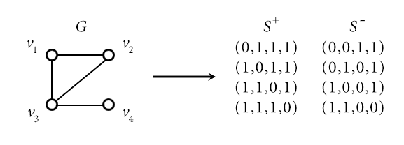
For a graph $ G$ with $ n$ nodes $ v_1, \dots, v_n$ and a set of $ m$ undirected edges $ E$, we construct a set of examples with positive labels $ S^+$ and one with negative examples $ S^-$. The examples are truth assignments to $ n$ variables, which we label $ x_1, \dots, x_n$, and we identify a truth assignment to the $ \left \{ 0,1 \right \}$-valued vector $ (x_1, x_2, \dots, x_n)$ in the usual way (true is 1, false is 0).

The positive examples $ S^+$ are simple: for each $ v_i$ add a truth assignment $ x_i = T, x_j = F$ for $ j \neq i$. I.e., the binary vector is $ (1, \dots, 1,0,1, \dots, 1)$, and the zero is in the $ i$-th position.

The negative examples $ S^-$ come from the edges. For each edge $ (v_i, v_j) \in E$, we add the example with a zero in the $ i$-th and $ j$-th components and ones everywhere else. Here is an example graph and the corresponding positive and negative examples:

Claim: $ G$ is 3-colorable if and only if the corresponding examples are consistent with some 3-term DNF formula $ \varphi$.

Again, consistent just means that $ \varphi$ is satisfied by every truth assignment in $ S^+$ and unsatisfied by every example in $ S^-$. Since we chose our distribution to be uniform over $ S^+ \cup S^-$, we don’t care what $ \varphi$ does elsewhere.

Indeed, if $ G$ is three-colorable we can fix some valid 3-coloring with colors red, blue, and yellow. We can construct a 3-term DNF that does what we need. Let $ T_R$ be the AND of all the literals $ x_i$ for which vertex $ v_i$ is not red. For each such $ i$, the corresponding example in $ S^+$ will satisfy $ T_R$, because we put a zero in the $ i$-th position and ones everywhere else. Similarly, no example in $ S^-$ will make $ T_R$ true because to do so both vertices in the corresponding edge would have to be red.

To drive this last point home say there are three vertices and your edge is $ (v_1,v_2)$. Then the corresponding negative example is $ (0,0,1)$. Unless both $ v_1$ and $ v_2$ are colored red, one of $ x_1, x_2$ will have to be ANDed as part of $ T_R$. But the example has a zero for both $ x_1$ and $ x_2$, so $ T_R$ would not be satisfied.

Doing the same thing for blue and yellow, and OR them together to get $ T_R \vee T_B \vee T_Y$. Since the case is symmetrically the same for the other colors, we a consistent 3-term DNF.

On the other hand, say there is a consistent 3-term DNF $ \varphi$. We need to construct a three coloring of $ G$. It goes in largely the same way: label the clauses $ \varphi = T_R \vee T_B \vee T_Y$ for Red, Blue, and Yellow, and then color a vertex $ v_i$ the color of the clause that is satisfied by the corresponding example in $ S^+$. There must be some clause that does this because $ \varphi$ is consistent with $ S^+$, and if there are multiple you can pick a valid color arbitrarily. Now we argue why no edge can be monochromatic. Suppose there were such an edge $ (v_i, v_j)$, and both $ v_i$ and $ v_j$ are colored, say, blue. Look at the clause $ T_B$: since $ v_i$ and $ v_j$ are both blue, the positive examples corresponding to those vertices (with a 0 in the single index and 1’s everywhere else) both make $ T_B$ true. Since those two positive examples differ in both their $ i$-th and $ j$-th positions, $ T_B$ can’t have any of the literals $ x_i, \overline{x_i}, x_j, \overline{x_j}$. But then the negative example for the edge would satisfy $ T_B$ because it has 1’s everywhere except $ i,j$! This means that the formula doesn’t consistently classify the negative examples, a contradiction. This proves the Claim.

Now we just need to show a few more details to finish the proof. In particular, we need to observe that the number of examples we generate is polynomial in the size of the graph $ G$; that the learning algorithm would still run in polynomial time in the size of the input graph (indeed, this depends on our choice of the learning parameters); and that we only need to pick $ \delta < 1/2$ and $ \varepsilon \leq 1/(2|S^+ \cup S^-|)$ in order to enforce that an efficient PAC-learner would generate a hypothesis consistent with all the examples. Indeed, if a hypothesis errs on even one example, it will have error at least $ 1 / |S^+ \cup S^-|$, which is too big.

Everything’s not Lost

This might seem a bit depressing for PAC-learning, that we can’t even hope to learn 3-term DNF formulas. But we will give a sketch of why this is mostly not a problem with PAC but a problem with DNFs.

In particular, the difficulty comes in forcing a PAC-learning algorithm to express its hypothesis as a 3-term DNF, as opposed to what we might argue is a more natural representation. As we observed, distributing the ORs in a 3-term DNF produces a 3-CNF formula (an AND of clauses where each clause is an OR of exactly three literals). Indeed, one can PAC-learn 3-CNF formulas efficiently, and it suffices to show that one can learn formulas which are just ANDs of literals. Then you can blow up the number of variables only polynomially larger to get 3-CNFs. ANDs of literals are just called “conjunctions,” so the problem is to PAC-learn conjunctions. The idea that works is the same one as in our first post on PAC where we tried to learn intervals: just pick the “smallest” hypothesis that is consistent with all the examples you’ve seen so far. We leave a formal proof as an (involved) exercise to the reader.

The important thing to note is that a concept class $ C$ (the thing we’re trying to learn) might be hard to learn if you’re constrained to work within $ C$. If you’re allowed more expressive hypotheses (in this case, arbitrary boolean formulas), then learning $ C$ suddenly becomes tractable. This compels us to add an additional caveat to the PAC definition from our first post.

Definition: A concept class $ \mathsf{C}$ over a set $ X$ is efficiently PAC-learnable using the hypothesis class $ \mathsf{H}$ if there exists an algorithm $ A(\varepsilon, \delta)$ with access to a query function for $ \mathsf{C}$ and runtime $ O(\text{poly}(1/\varepsilon, 1/\delta))$, such that for all $ c \in \mathsf{C}$, all distributions $ D$ over $ X$, and all $ 0 < \delta , \varepsilon < 1/2$, the probability that $ A$ produces a hypothesis $ h \in \mathsf{H}$ with error at most $ \varepsilon$ is at least $ 1-\delta$.

And with that we’ll end this extended side note. The next post in this series will introduce and analyze a fascinating notion of dimension for concept classes, the Vapnik-Chervonenkis dimension.

Until then!