Graphs are among the most interesting and useful objects in mathematics. Any situation or idea that can be described by objects with connections is a graph, and one of the most prominent examples of a real-world graph that one can come up with is a social network.
Recall, if you aren’t already familiar with this blog’s gentle introduction to graphs, that a graph $ G$ is defined by a set of vertices $ V$, and a set of edges $ E$, each of which connects two vertices. For this post the edges will be undirected, meaning connections between vertices are symmetric.
One of the most common topics to talk about for graphs is the notion of a community. But what does one actually mean by that word? It’s easy to give an informal definition: a subset of vertices $ C$ such that there are many more edges between vertices in $ C$ than from vertices in $ C$ to vertices in $ V – C$ (the complement of $ C$). Try to make this notion precise, however, and you open a door to a world of difficult problems and open research questions. Indeed, nobody has yet come to a conclusive and useful definition of what it means to be a community. In this post we’ll see why this is such a hard problem, and we’ll see that it mostly has to do with the word “useful.” In future posts we plan to cover some techniques that have found widespread success in practice, but this post is intended to impress upon the reader how difficult the problem is.
The simplest idea
The simplest thing to do is to say a community is a subset of vertices which are completely connected to each other. In the technical parlance, a community is a subgraph which forms a clique. Sometimes an $ n$-clique is also called a complete graph on $ n$ vertices, denoted $ K_n$. Here’s an example of a 5-clique in a larger graph:
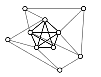
'Where's Waldo' for graph theorists: a clique hidden in a larger graph.
Indeed, it seems reasonable that if we can reliably find communities at all, then we should be able to find cliques. But as fate should have it, this problem is known to be computationally intractable. In more detail, the problem of finding the largest clique in a graph is NP-hard. That essentially means we don’t have any better algorithms to find cliques in general graphs than to try all possible subsets of the vertices and check to see which, if any, form cliques. In fact it’s much worse, this problem is known to be hard to approximate to any reasonable factor in the worst case (the error of the approximation grows polynomially with the size of the graph!). So we can’t even hope to find a clique half the size of the biggest, or a thousandth the size!
But we have to take these impossibility results with a grain of salt: they only say things about the worst case graphs. And when we’re looking for communities in the real world, the worst case will never show up. Really, it won’t! In these proofs, “worst case” means that they encode some arbitrarily convoluted logic problem into a graph, so that finding the clique means solving the logic problem. To think that someone could engineer their social network to encode difficult logic problems is ridiculous.
So what about an “average case” graph? To formulate this typically means we need to consider graphs randomly drawn from a distribution.
Random graphs
The simplest kind of “randomized” graph you could have is the following. You fix some set of vertices, and then run an experiment: for each pair of vertices you flip a coin, and if the coin is heads you place an edge and otherwise you don’t. This defines a distribution on graphs called $ G(n, 1/2)$, which we can generalize to $ G(n, p)$ for a coin with bias $ p$. With a slight abuse of notation, we call $ G(n, p)$ the Erdős–Rényi random graph (it’s not a graph but a distribution on graphs). We explored this topic form a more mathematical perspective earlier on this blog.
So we can sample from this distribution and ask questions like: what’s the probability of the largest clique being size at least $ 20$? Indeed, cliques in Erdős–Rényi random graphs are so well understood that we know exactly how they work. For example, if $ p=1/2$ then the size of the largest clique is guaranteed (with overwhelming probability as $ n$ grows) to have size $ k(n)$ or $ k(n)+1$, where $ k(n)$ is about $ 2 \log n$. Just as much is known about other values of $ p$ as well as other properties of $ G(n,p)$, see Wikipedia for a short list.
In other words, if we wanted to find the largest clique in an Erdős–Rényi random graph, we could check all subsets of size roughly $ 2\log(n)$, which would take about $ (n / \log(n))^{\log(n)}$ time. This is pretty terrible, and I’ve never heard of an algorithm that does better (contrary to the original statement in this paragraph that showed I can’t count). In any case, it turns out that the Erdős–Rényi random graph, and using cliques to represent communities, is far from realistic. There are many reasons why this is the case, but here’s one example that fits with the topic at hand. If I thought the world’s social network was distributed according to $ G(n, 1/2)$ and communities were cliques, then I would be claiming that the largest community is of size 65 or 66. Estimated world population: 7 billion, $ 2 \log(7 \cdot 10^9) \sim 65$. Clearly this is ridiculous: there are groups of larger than 66 people that we would want to call “communities,” and there are plenty of communities that don’t form bona-fide cliques.
Another avenue shows that things are still not as easy as they seem in Erdős–Rényi land. This is the so-called planted clique problem. That is, you draw a graph $ G$ from $ G(n, 1/2)$. You give $ G$ to me and I pick a random but secret subset of $ r$ vertices and I add enough edges to make those vertices form an $ r$-clique. Then I ask you to find the $ r$-clique. Clearly it doesn’t make sense when $ r < 2 \log (n) $ because you won’t be able to tell it apart from the guaranteed cliques in $ G$. But even worse, nobody knows how to find the planted clique when $ r$ is even a little bit smaller than $ \sqrt{n}$ (like, $ r = n^{9/20}$ even). Just to solidify this with some numbers, we don’t know how to reliably find a planted clique of size 60 in a random graph on ten thousand vertices, but we do when the size of the clique goes up to 100. The best algorithms we know rely on some sophisticated tools in spectral graph theory, and their details are beyond the scope of this post.
So Erdős–Rényi graphs seem to have no hope. What’s next? There are a couple of routes we can take from here. We can try to change our random graph model to be more realistic. We can relax our notion of communities from cliques to something else. We can do both, or we can do something completely different.
Other kinds of random graphs
There is an interesting model of Barabási and Albert, often called the “preferential attachment” model, that has been described as a good model of large, quickly growing networks like the internet. Here’s the idea: you start off with a two-clique $ G = K_2$, and at each time step $ t$ you add a new vertex $ v$ to $ G$, and new edges so that the probability that the edge $ (v,w)$ is added to $ G$ is proportional to the degree of $ w$ (as a fraction of the total number of edges in $ G$). Here’s an animation of this process:

Image source: Wikipedia
The significance of this random model is that it creates graphs with a small number of hubs, and a large number of low-degree vertices. In other words, the preferential attachment model tends to “make the rich richer.” Another perspective is that the degree distribution of such a graph is guaranteed to fit a so-called power-law distribution. Informally, this means that the overall fraction of small-degree vertices gives a significant contribution to the total number of edges. This is sometimes called a “fat-tailed” distribution. Since power-law distributions are observed in a wide variety of natural settings, some have used this as justification for working in the preferential attachment setting. On the other hand, this model is known to have no significant community structure (by any reasonable definition, certainly not having cliques of nontrivial size), and this has been used as evidence against the model. I am not aware of any work done on planting dense subgraphs in graphs drawn from a preferential attachment model, but I think it’s likely to be trivial and uninteresting. On the other hand, Bubeck et al. have looked at changing the initial graph (the “seed”) from a 2-clique to something else, and seeing how that affects the overall limiting distribution.
Another model that often shows up is a model that allows one to make a random graph starting with any fixed degree distribution, not just a power law. There are a number of models that do this to some fashion, and you’ll hear a lot of hyphenated names thrown around like Chung-Lu and Molloy-Reed and Newman-Strogatz-Watts. The one we’ll describe is quite simple. Say you start with a set of vertices $ V$, and a number $ d_v$ for each vertex $ v$, such that the sum of all the $ d_v$ is even. This condition is required because in any graph the sum of the degrees of a vertex is twice the number of edges. Then you imagine each vertex $ v$ having $ d_v$ “edge-stubs.” The name suggests a picture like the one below:
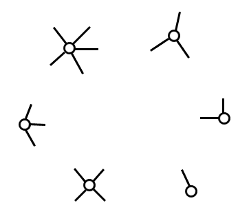
Each node has a prescribed number of 'edge stubs,' which are randomly connected to form a graph.
Now you pick two edge stubs at random and connect them. One usually allows self-loops and multiple edges between vertices, so that it’s okay to pick two edge stubs from the same vertex. You keep doing this until all the edge stubs are accounted for, and this is your random graph. The degrees were fixed at the beginning, so the only randomization is in which vertices are adjacent. The same obvious biases apply, that any given vertex is more likely to be adjacent to high-degree vertices, but now we get to control the biases with much more precision.
The reason such a model is useful is that when you’re working with graphs in the real world, you usually have statistical information available. It’s simple to compute the degree of each vertex, and so you can use this random graph as a sort of “prior” distribution and look for anomalies. In particular, this is precisely how one of the leading measures of community structure works: the measure of modularity. We’ll talk about this in the next section.
Other kinds of communities
Here’s one easy way to relax our notion of communities. Rather than finding complete subgraphs, we could ask about finding very dense subgraphs (ignoring what happens outside the subgraph). We compute density as the average degree of vertices in the subgraph.
If we impose no bound on the size of the subgraph an algorithm is allowed to output, then there is an efficient algorithm for finding the densest subgraph in a given graph. The general exact solution involves solving a linear programming problem and a little extra work, but luckily there is a greedy algorithm that can get within half of the optimal density. You start with all the vertices $ S_n = V$, and remove any vertex of minimal degree to get $ S_{n-1}$. Continue until $ S_0$, and then compute the density of all the $ S_i$. The best one is guaranteed to be at least half of the optimal density. See this paper of Moses Charikar for a more formal analysis.
One problem with this is that the size of the densest subgraph might be too big. Unfortunately, if you fix the size of the dense subgraph you’re looking for (say, you want to find the densest subgraph of size at most $ k$ where $ k$ is an input), then the problem once again becomes NP-hard and suffers from the same sort of inapproximability theorems as finding the largest clique.
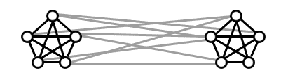
A more important issue with this is that a dense subgraph isn’t necessarily a community. In particular, we want communities to be dense on the inside and sparse on the outside. The densest subgraph analysis, however, might rate the following graph as one big dense subgraph instead of two separately dense communities with some modest (but not too modest) amount of connections between them.
What should be identified as communities?
Indeed, we want a quantifiable a notion of “dense on the inside and sparse on the outside.” One such formalization is called modularity. Modularity works as follows. If you give me some partition of the vertices of $ G$ into two sets, modularity measures how well this partition reflects two separate communities. It’s the definition of “community” here that makes it interesting. Rather than ask about densities exactly, you can compare the densities to the expected densities in a given random graph model.
In particular, we can use the fixed-degree distribution model from the last section. If we know the degrees of all the vertices ahead of time, we can compute the probability that we see some number of edges going between the two pieces of the partition relative to what we would see at random. If the difference is large (and largely biased toward fewer edges across the partition and more edges within the two subsets), then we say it has high modularity. This involves a lot of computations — the whole measure can be written as a quadratic form via one big matrix — but the idea is simple enough. We intend to write more about modularity and implement the algorithm on this blog, but the excited reader can see the original paper of M.E.J. Newman.
Now modularity is very popular but it too has shortcomings. First, even though you can compute the modularity of a given partition, there’s still the problem of finding the partition that globally maximizes modularity. Sadly, this is known to be NP-hard. Mover, it’s known to be NP-hard even if you’re just trying to find a partition into two pieces that maximizes modularity, and even still when the graph is regular (every vertex has the same degree).
Still worse, while there are some readily accepted heuristics that often “do well enough” in practice, we don’t even know how to approximate modularity very well. Bhaskar DasGupta has a line of work studying approximations of maximum modularity, and he has proved that for dense graphs you can’t even approximate modularity to within any constant factor. That is, the best you can do is have an approximation that gets worse as the size of the graph grows. It’s similar to the bad news we had for finding the largest clique, but not as bad. For example, when the graph is sparse it’s known that one can approximate modularity to within a $ \log(n)$ factor of the optimum, where $ n$ is the number of vertices of the graph (for cliques the factor was like $ n^c$ for some $ c$, and this is drastically worse).
Another empirical issue is that modularity seems to fail to find small communities. That is, if your graph has some large communities and some small communities, strictly maximizing the modularity is not the right thing to do. So we’ve seen that even the leading method in the field has some issues.
Something completely different
The last method I want to sketch is in the realm of “something completely different.” The notion is that if we’re given a graph, we can run some experiment on the graph, and the results of that experiment can give us insight into where the communities are.
The experiment I’m going to talk about is the random walk. That is, say you have a vertex $ v$ in a graph $ G$ and you want to find some vertices that are “closest” to $ v$. That is, those that are most likely to be in the same community as $ v$. What you can do is run a random walk starting at $ v$. By a “random walk” I mean you start at $ v$, you pick a neighbor at random and move to it, then repeat. You can compute statistics about the vertices you visit in a sample of such walks, and the vertices that you visit most often are those you say are “in the same community as $ v$. One important parameter is how long the walk is, but it’s generally believed to be best if you keep it between 3-6 steps.
Of course, this is not a partition of the vertices, so it’s not a community detection algorithm, but you can turn it into one. Run this process for each vertex, and use it to compute a “distance” between all the pairs of vertices. Then you compute a tree of partitions by lumping the closest pairs of vertices into the same community, one at a time, until you’ve got every vertex. At each step of the way, you compute the modularity of the partition, and when you’re done you choose the partition that maximizes modularity. This algorithm as a whole is called the walktrap clustering algorithm, and was introduced by Pons and Latapy in 2005.
This sounds like a really great idea, because it’s intuitive: there’s a relatively high chance that the friends of your friends are also your friends. It’s also really great because there is an easily measurable tradeoff between runtime and quality: you can tune down the length of the random walk, and the number of samples you take for each vertex, to speed up the runtime but lower the quality of your statistical estimates. So if you’re working on huge graphs, you get a lot of control and a clear idea of exactly what’s going on inside the algorithm (something which is not immediately clear in a lot of these papers).
Unfortunately, I’m not aware of any concrete theoretical guarantees for walktrap clustering. The one bit of theoretical justification I’ve read over the last year is that you can relate the expected distances you get to certain spectral properties of the graph that are known to be related to community structure, but the lower bounds on maximizing modularity already suggest (though they do not imply) that walktrap won’t do that well in the worst case.
So many algorithms, so little time!
I have only brushed the surface of the literature on community detection, and the things I have discussed are heavily biased toward what I’ve read about and used in my own research. There are methods based on information theory, label propagation, and obscure physics processes like “spin glass” (whatever that is, it sounds frustrating).
And we have only been talking about perfect community structure. What if you want to allow people to be in multiple communities, or have communities at varying levels of granularity (e.g. a sports club within a school versus the whole student body of that school)? What if we want to allow people to be “members” of a community at varying degrees of intensity? How do we deal with noisy signals in our graphs? For example, if we get our data from observing people talk, are two people who have heated arguments considered to be in the same community? Since a lot social network data comes from sources like Twitter and Facebook where arguments are rampant, how do we distinguish between useful and useless data? More subtly, how do we determine useful information if a group within the social network are trying to mask their discovery? That is, how do we deal with adversarial noise in a graph?
And all of this is just on static graphs! What about graphs that change over time? You can keep making the problem more and more complicated as it gets more realistic.
With the huge wealth of research that has already been done just on the simplest case, and the difficult problems and known barriers to success even for the simple problems, it seems almost intimidating to even begin to try to answer these questions. But maybe that’s what makes them fascinating, not to mention that governments and big businesses pour many millions of dollars into this kind of research.
In the future of this blog we plan to derive and implement some of the basic methods of community detection. This includes, as a first outline, the modularity measure and the walktrap clustering algorithm. Considering that I’m also going to spend a large part of the summer thinking about these problems (indeed, with some of the leading researchers and upcoming stars under the sponsorship of the American Mathematical Society), it’s unlikely to end there.
Until next time!
Want to respond? Send me an email, post a webmention, or find me elsewhere on the internet.