Optimization is by far one of the richest ways to apply computer science and mathematics to the real world. Everybody is looking to optimize something: companies want to maximize profits, factories want to maximize efficiency, investors want to minimize risk, the list just goes on and on. The mathematical tools for optimization are also some of the richest mathematical techniques. They form the cornerstone of an entire industry known as operations research, and advances in this field literally change the world.
The mathematical field is called combinatorial optimization, and the name comes from the goal of finding optimal solutions more efficiently than an exhaustive search through every possibility. This post will introduce the most central problem in all of combinatorial optimization, known as the linear program. Even better, we know how to efficiently solve linear programs, so in future posts we’ll write a program that computes the most affordable diet while meeting the recommended health standard.
Generalizing a Specific Linear Program
Most optimization problems have two parts: an objective function, the thing we want to maximize or minimize, and constraints, rules we must abide by to ensure we get a valid solution. As a simple example you may want to minimize the amount of time you spend doing your taxes (objective function), but you certainly can’t spend a negative amount of time on them (a constraint).
The following more complicated example is the centerpiece of this post. Most people want to minimize the amount of money spent on food. At the same time, one needs to maintain a certain level of nutrition. For males ages 19-30, the United States National Institute for Health recommends 3.7 liters of water per day, 1,000 milligrams of calcium per day, 90 milligrams of vitamin C per day, etc.
We can set up this nutrition problem mathematically, just using a few toy variables. Say we had the option to buy some combination of oranges, milk, and broccoli. Some rough estimates [1] give the following content/costs of these foods. For 0.272 USD you can get 100 grams of orange, containing a total of 53.2mg of calcium, 40mg of vitamin C, and 87g of water. For 0.100 USD you can get 100 grams of whole milk, containing 276mg of calcium, 0mg of vitamin C, and 87g of water. Finally, for 0.381 USD you can get 100 grams of broccoli containing 47mg of calcium, 89.2mg of vitamin C, and 91g of water. Here’s a table summarizing this information:
Nutritional content and prices for 100g of three foods

Food         calcium(mg)     vitamin C(mg)      water(g)   price(USD/100g)
Broccoli     47              89.2               91         0.381
Whole milk   276             0                  87         0.100
Oranges      40              53.2               87         0.272
Some observations: broccoli is more expensive but gets the most of all three nutrients, whole milk doesn’t have any vitamin C but gets a ton of calcium for really cheap, and oranges are a somewhere in between. So you could probably tinker with the quantities and figure out what the cheapest healthy diet is. The problem is what happens when we incorporate hundreds or thousands of food items and tens of nutrient recommendations. This simple example is just to help us build up a nice formality.
So let’s continue doing that. If we denote by $ b$ the number of 100g units of broccoli we decide to buy, and $ m$ the amount of milk and $ r$ the amount of oranges, then we can write the daily cost of food as
$$\displaystyle \text{cost}(b,m,r) = 0.381 b + 0.1 m + 0.272 r$$In the interest of being compact (and again, building toward the general linear programming formulation) we can extract the price information into a single cost vector $ c = (0.381, 0.1, 0.272)$, and likewise write our variables as a vector $ x = (b,m,r)$. We’re implicitly fixing an ordering on the variables that is maintained throughout the problem, but the choice of ordering doesn’t matter. Now the cost function is just the inner product (dot product) of the cost vector and the variable vector $ \left \langle c,x \right \rangle$. For some reason lots of people like to write this as $ c^Tx$, where $ c^T$ denotes the transpose of a matrix, and we imagine that $ c$ and $ x$ are matrices of size $ 3 \times 1$. I’ll stick to using the inner product bracket notation.
Now for each type of food we get a specific amount of each nutrient, and the sum of those nutrients needs to be bigger than the minimum recommendation. For example, we want at least 1,000 mg of calcium per day, so we require that $ 1000 \leq 47b + 276m + 40r$. Likewise, we can write out a table of the constraints by looking at the columns of our table above.
$$\displaystyle \begin{matrix} 91b & + & 87m & + & 87r & \geq & 3700 & \text{(water)}\\\ 47b & + & 276m & + & 40r & \geq & 1000 & \text{(calcium)} \\\ 89.2b & + & 0m & + & 53.2r & \geq & 90 & \text{(vitamin C)} \end{matrix}$$In the same way that we extracted the cost data into a vector to separate it from the variables, we can extract all of the nutrient data into a matrix $ A$, and the recommended minimums into a vector $ v$. Traditionally the letter $ b$ is used for the minimums vector, but for now we’re using $ b$ for broccoli.
$$A = \begin{pmatrix} 91 & 87 & 87 \\\ 47 & 276 & 40 \\\ 89.2 & 0 & 53.2 \end{pmatrix}$$ $$v = \begin{pmatrix} 3700 \\\ 1000 \\\ 90 \end{pmatrix}$$And now the constraint is that $ Ax \geq v$, where the $ \geq$ means “greater than or equal to in every coordinate.” So now we can write down the more general form of the problem for our specific matrices and vectors. That is, our problem is to minimize $ \left \langle c,x \right \rangle$ subject to the constraint that $ Ax \geq v$. This is often written in offset form to contrast it with variations we’ll see in a bit:
$$\displaystyle \text{minimize} \left \langle c,x \right \rangle \\\ \text{subject to the constraint } Ax \geq v$$In general there’s no reason you can’t have a “negative” amount of one variable. In this problem you can’t buy negative broccoli, so we’ll add the constraints to ensure the variables are nonnegative. So our final form is
$$\displaystyle \text{minimize} \left \langle c,x \right \rangle \\\ \text{subject to } Ax \geq v \\\ \text{and } x \geq 0$$In general, if you have an $ m \times n$ matrix $ A$, a “minimums” vector $ v \in \mathbb{R}^m$, and a cost vector $ c \in \mathbb{R}^n$, the problem of finding the vector $ x$ that minimizes the cost function while meeting the constraints is called a linear programming problem or simply a linear program.
To satiate the reader’s burning curiosity, the solution for our calcium/vitamin C problem is roughly $ x = (1.01, 41.47, 0)$. That is, you should have about 100g of broccoli and 4.2kg of milk (like 4 liters), and skip the oranges entirely. The daily cost is about 4.53 USD. If this seems awkwardly large, it’s because there are cheaper ways to get water than milk.

100-grams-broccoli
[1] Water content of fruits and veggies, Food costs in March 2014 in the midwest, and basic known facts about the water density/nutritional content of various foods.
Duality
Now that we’ve seen the general form a linear program and a cute example, we can ask the real meaty question: is there an efficient algorithm that solves arbitrary linear programs? Despite how widely applicable these problems seem, the answer is yes!
But before we can describe the algorithm we need to know more about linear programs. For example, say you have some vector $ x$ which satisfies your constraints. How can you tell if it’s optimal? Without such a test we’d have no way to know when to terminate our algorithm. Another problem is that we’ve phrased the problem in terms of minimization, but what about problems where we want to maximize things? Can we use the same algorithm that finds minima to find maxima as well?
Both of these problems are neatly answered by the theory of duality. In mathematics in general, the best way to understand what people mean by “duality” is that one mathematical object uniquely determines two different perspectives, each useful in its own way. And typically a duality theorem provides one with an efficient way to transform one perspective into the other, and relate the information you get from both perspectives. A theory of duality is considered beautiful because it gives you truly deep insight into the mathematical object you care about.
In linear programming duality is between maximization and minimization. In particular, every maximization problem has a unique “dual” minimization problem, and vice versa. The really interesting thing is that the variables you’re trying to optimize in one form correspond to the contraints in the other form! Here’s how one might discover such a beautiful correspondence. We’ll use a made up example with small numbers to make things easy.
So you have this optimization problem
$ \displaystyle \begin{matrix} \text{minimize} & 4x_1+3x_2+9x_3 & \\\ \text{subject to} & x_1+x_2+x_3 & \geq 6 \\\ & 2x_1+x_3 & \geq 2 \\\ & x_2+x_3 & \geq 1 & \\\ & x_1,x_2,x_3 & \geq 0 \end{matrix}$
Just for giggles let’s write out what $ A$ and $ c$ are.
$$\displaystyle A = \begin{pmatrix} 1 & 1 & 1 \\\ 2 & 0 & 1 \\\ 0 & 1 & 1 \end{pmatrix}, c = (4,3,9), v = (6,2,1)$$Say you want to come up with a lower bound on the optimal solution to your problem. That is, you want to know that you can’t make $ 4x_1 + 3x_2 + 9x_3$ smaller than some number $ m$. The constraints can help us derive such lower bounds. In particular, every variable has to be nonnegative, so we know that $ 4x_1 + 3x_2 + 9x_3 \geq x_1 + x_2 + x_3 \geq 6$, and so 6 is a lower bound on our optimum. Likewise,
$$\displaystyle \begin{aligned}4x_1+3x_2+9x_3 & \geq 4x_1+4x_3+3x_2+3x_3 \\\ &=2(2x_1 + x_3)+3(x_2+x_3) \\\ & \geq 2 \cdot 2 + 3 \cdot 1 \\\ &=7\end{aligned}$$and that’s an even better lower bound than 6. We could try to write this approach down in general: find some numbers $ y_1, y_2, y_3$ that we’ll use for each constraint to form
$$\displaystyle y_1(\text{constraint 1}) + y_2(\text{constraint 2}) + y_3(\text{constraint 3})$$To make it a valid lower bound we need to ensure that the coefficients of each of the $ x_i$ are smaller than the coefficients in the objective function (i.e. that the coefficient of $ x_1$ ends up less than 4). And to make it the best lower bound possible we want to maximize what the right-hand-size of the inequality would be: $ y_1 6 + y_2 2 + y_3 1$. If you write out these equations and the constraints you get our “lower bound” problem written as
$$\displaystyle \begin{matrix} \text{maximize} & 6y_1 + 2y_2 + y_3 & \\\ \text{subject to} & y_1 + 2y_2 & \leq 4 \\\ & y_1 + y_3 & \leq 3 \\\ & y_1+y_2 + y_3 & \leq 9 \\\ & y_1,y_2,y_3 & \geq 0 \end{matrix}$$And wouldn’t you know, the matrix providing the constraints is $ A^T$, and the vectors $ c$ and $ v$ switched places.
$$\displaystyle A^T = \begin{pmatrix} 1 & 2 & 0 \\\ 1 & 0 & 1 \\\ 1 & 1 & 1 \end{pmatrix}$$This is no coincidence. All linear programs can be transformed in this way, and it would be a useful exercise for the reader to turn the above maximization problem back into a minimization problem by the same technique (computing linear combinations of the constraints to make upper bounds). You’ll be surprised to find that you get back to the original minimization problem! This is part of what makes it “duality,” because the dual of the dual is the original thing again. Often, when we fix the “original” problem, we call it the primal form to distinguish it from the dual form. Usually the primal problem is the one that is easy to interpret.
(Note: because we’re done with broccoli for now, we’re going to use $ b$ to denote the constraint vector that used to be $ v$.)
Now say you’re given the data of a linear program for minimization, that is the vectors $ c, b$ and matrix $ A$ for the problem, “minimize $ \left \langle c, x \right \rangle$ subject to $ Ax \geq b; x \geq 0$.” We can make a general definition: the dual linear program is the maximization problem “maximize $ \left \langle b, y \right \rangle$ subject to $ A^T y \leq c, y \geq 0$.” Here $ y$ is the new set of variables and the superscript T denotes the transpose of the matrix. The constraint for the dual is often written $ y^T A \leq c^T$, again identifying vectors with a single-column matrices, but I find the swamp of transposes pointless and annoying (why do things need to be columns?).
Now we can actually prove that the objective function for the dual provides a bound on the objective function for the original problem. It’s obvious from the work we’ve done, which is why it’s called the weak duality theorem.
Weak Duality Theorem: Let $ c, A, b$ be the data of a linear program in the primal form (the minimization problem) whose objective function is $ \left \langle c, x \right \rangle$. Recall that the objective function of the dual (maximization) problem is $ \left \langle b, y \right \rangle$. If $ x,y$ are feasible solutions (satisfy the constraints of their respective problems), then
$$\left \langle b, y \right \rangle \leq \left \langle c, x \right \rangle$$In other words, the maximum of the dual is a lower bound on the minimum of the primal problem and vice versa. Moreover, any feasible solution for one provides a bound on the other.
Proof. The proof is pleasingly simple. Just inspect the quantity $ \left \langle A^T y, x \right \rangle = \left \langle y, Ax \right \rangle$. The constraints from the definitions of the primal and dual give us that
$$\left \langle y, b \right \rangle \leq \left \langle y, Ax \right \rangle = \left \langle A^Ty, x \right \rangle \leq \left \langle c,x \right \rangle$$The inequalities follow from the linear algebra fact that if the $ u$ in $ \left \langle u,v \right \rangle$ is nonnegative, then you can only increase the size of the product by increasing the components of $ v$. This is why we need the nonnegativity constraints.
In fact, the world is much more pleasing. There is a theorem that says the two optimums are equal!
Strong Duality Theorem: If there are any solutions $ x,y$ to the primal (minimization) problem and the dual (maximization) problem, respectively, then the two problems also have optimal solutions $ x^*, y^*$, and two candidate solutions $ x^*, y^*$ are optimal if and only if they produce equal objective values $ \left \langle c, x^* \right \rangle = \left \langle y^*, b \right \rangle$.
The proof of this theorem is a bit more convoluted than the weak duality theorem, and the key technique is a lemma of Farkas and its variations. See the second half of these notes for a full proof. The nice thing is that this theorem gives us a way to tell if an algorithm to solve linear programs is done: maintain a pair of feasible solutions to the primal and dual problems, improve them by some rule, and stop when the two solutions give equal objective values. The hard part, then, is finding a principled and guaranteed way to improve a given pair of solutions.
On the other hand, you can also prove the strong duality theorem by inventing an algorithm that provably terminates. We’ll see such an algorithm, known as the simplex algorithm in the next post. Sneak peek: it’s a lot like Gaussian elimination. Then we’ll use the algorithm (or an equivalent industry-strength version) to solve a much bigger nutrition problem.
In fact, you can do a bit better than the strong duality theorem, in terms of coming up with a stopping condition for a linear programming algorithm. You can observe that an optimal solution implies further constraints on the relationship between the primal and the dual problems. In particular, this is called the complementary slackness conditions, and they essentially say that if an optimal solution to the primal has a positive variable then the corresponding constraint in the dual problem must be tight (is an equality) to get an optimal solution to the dual. The contrapositive says that if some constraint is slack, or a strict inequality, then either the corresponding variable is zero or else the solution is not optimal. More formally,
Theorem (Complementary Slackness Conditions): Let $ A, c, b$ be the data of the primal form of a linear program, “minimize $ \left \langle c, x \right \rangle$ subject to $ Ax \geq b, x \geq 0$.” Then $ x^*, y^*$ are optimal solutions to the primal and dual problems if any only if all of the following conditions hold.
- $ x^*, y^*$ are both feasible for their respective problems.
- Whenever $ x^*_i > 0$ the corresponding constraint $ A^T_i y^* = c_i$ is an equality.
- Whenever $ y^*_j > 0$ the corresponding constraint $ A_j x^* = b_j$ is an equality.
Here we denote by $ M_i$ the $ i$-th row of the matrix $ M$ and $ v_i$ to denote the $ i$-th entry of a vector. Another way to write the condition using vectors instead of English is
$ \left \langle x^*, A^T y^* – c \right \rangle = 0$
$$\left \langle y^*, Ax^* – b \right \rangle$$The proof follows from the duality theorems, and just involves pushing around some vector algebra. See section 6.2 of these notes.
One can interpret complementary slackness in linear programs in a lot of different ways. For us, it will simply be a termination condition for an algorithm: one can efficiently check all of these conditions for the nonzero variables and stop if they’re all satisfied or if we find a variable that violates a slackness condition. Indeed, in more mature optimization analyses, the slackness condition that is more egregiously violated can provide evidence for where a candidate solution can best be improved. For a more intricate and detailed story about how to interpret the complementary slackness conditions, see Section 4 of these notes by Joel Sobel.
Finally, before we close we should note there are geometric ways to think about linear programming. I have my preferred visualization in my head, but I have yet to find a suitable animation on the web that replicates it. Here’s one example in two dimensions. The set of constraints define a convex geometric region in the plane
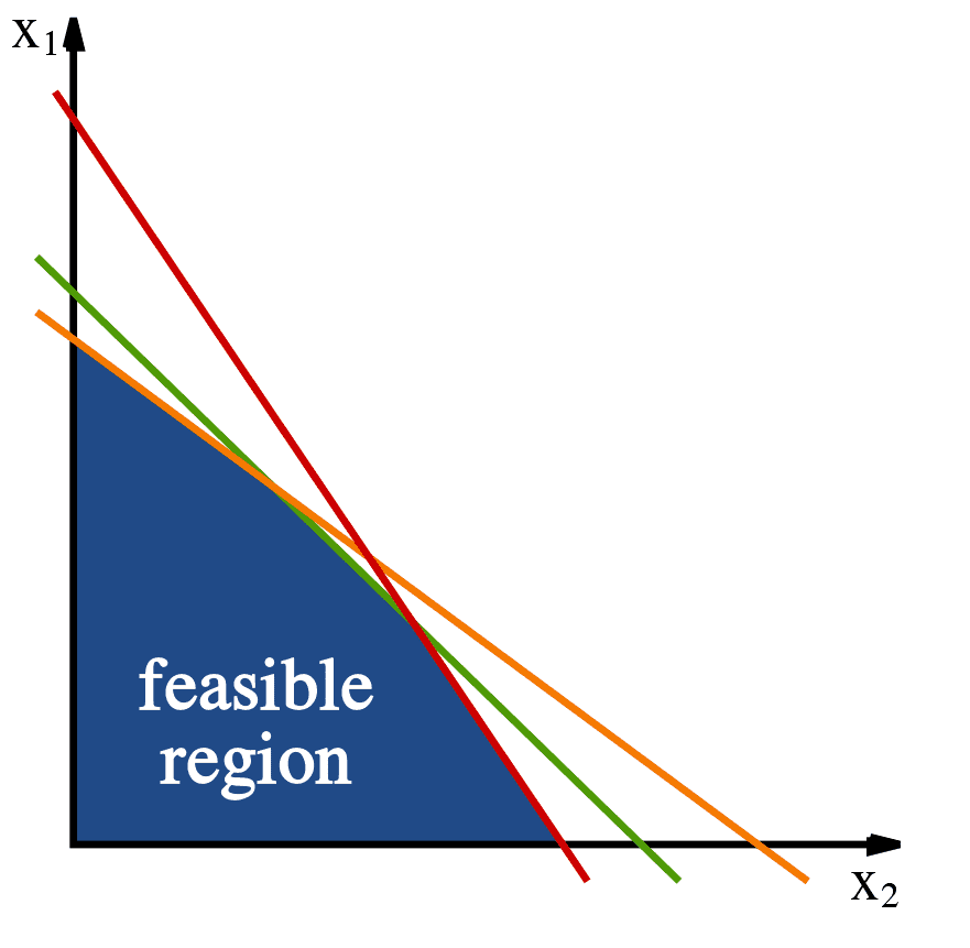
The constraints define a convex area of 'feasible solutions.' Image source: Wikipedia.
Now the optimization function $ f(x) = \left \langle c,x \right \rangle$ is also a linear function, and if you fix some output value $ y = f(x)$ this defines a line in the plane. As $ y$ changes, the line moves along its normal vector (that is, all these fixed lines are parallel). Now to geometrically optimize the target function, we can imagine starting with the line $ f(x) = 0$, and sliding it along its normal vector in the direction that keeps it in the feasible region. We can keep sliding it in this direction, and the maximum of the function is just the last instant that this line intersects the feasible region. If none of the constraints are parallel to the family of lines defined by $ f$, then this is guaranteed to occur at a vertex of the feasible region. Otherwise, there will be a family of optima lying anywhere on the line segment of last intersection.
In higher dimensions, the only change is that the lines become affine subspaces of dimension $ n-1$. That means in three dimensions you’re sliding planes, in four dimensions you’re sliding 3-dimensional hyperplanes, etc. The facts about the last intersection being a vertex or a “line segment” still hold. So as we’ll see next time, successful algorithms for linear programming in practice take advantage of this observation by efficiently traversing the vertices of this convex region. We’ll see this in much more detail in the next post.
Until then!
Want to respond? Send me an email, post a webmention, or find me elsewhere on the internet.