Greedy algorithms are among the simplest and most intuitive algorithms known to humans. Their name essentially gives their description: do the thing that looks best right now, and repeat until nothing looks good anymore or you’re forced to stop. Some of the best situations in computer science are also when greedy algorithms are optimal or near-optimal. There is a beautiful theory of this situation, known as the theory of matroids. We haven’t covered matroids on this blog (edit: we did), but in this post we will focus on the next best thing: when the greedy algorithm guarantees a reasonably good approximation to the optimal solution.
This situation isn’t hard to formalize, and we’ll make it as abstract as possible. Say you have a set of objects $ X$, and you’re looking to find the “best” subset $ S \subset X$. Here “best” is just measured by a fixed (known, efficiently computable) objective function $ f : 2^X \to \mathbb{R}$. That is, $ f$ accepts as input subsets of $ X$ and outputs numbers so that better subsets have larger numbers. Then the goal is to find a subset maximizing $ f$.
In this generality the problem is clearly impossible. You’d have to check all subsets to be sure you didn’t miss the best one. So what conditions do we need on either $ X$ or $ f$ or both that makes this problem tractable? There are plenty you could try, but one very rich property is submodularity.
The Submodularity Condition
I think the simplest way to explain submodularity is in terms of coverage. Say you’re starting a new radio show and you have to choose which radio stations to broadcast from to reach the largest number of listeners. For simplicity say each radio station has one tower it broadcasts from, and you have a good estimate of the number of listeners you would reach if you broadcast from a given tower. For more simplicity, say it costs the same to broadcast from each tower, and your budget restricts you to a maximum of ten stations to broadcast from. So the question is: how do you pick towers to maximize your overall reach?
The hidden condition here is that some towers overlap in which listeners they reach. So if you broadcast from two towers in the same city, a listener who has access to both will just pick one or the other. In other words, there’s a diminished benefit to picking two overlapping towers if you already have chosen one.
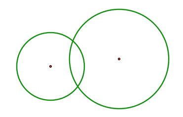
In our version of the problem, picking both of these towers has some small amount of 'overkill.'
This “diminishing returns” condition is a general idea you can impose on any function that takes in subsets of a given set and produces numbers. If $ X$ is a set, then for a strange reason we denote by $ 2^X$ the set of all subsets of $ X$. So we can state this condition more formally,
Definition: Let $ X$ be a finite set. A function $ f: 2^X \to \mathbb{R}$ is called submodular if for all subsets $ S \subset T \subset X$ and all $ x \in X \setminus T$,
$$\displaystyle f(S \cup \{ x \}) – f(S) \geq f(T \cup \{ x \}) – f(T)$$In other words, if $ f$ measures “benefit,” then the marginal benefit of adding $ x$ to $ S$ is at least as high as the marginal benefit of adding it to $ T$. Since $ S \subset T$ and $ x$ are all arbitrary, this is as general as one could possibly make it: adding $ x$ to a bigger set can’t be better than adding it to a smaller set.
Before we start doing things with submodular functions, let’s explore some basic properties. The first is an equivalent definition of submodularity
Proposition: $ f$ is submodular if and only if for all $ A, B \subset X$, it holds that
$ \displaystyle f(A \cap B) + f(A \cup B) \leq f(A) + f(B)$.
Proof. If we assume $ f$ has the condition from this proposition, then we can set $ A=T, B=S \cup \{ x \}$, and the formula just works out. Conversely, if we have the condition from the definition, then using the fact that $ A \cap B \subset B$ we can inductively apply the inequality to each element of $ A \setminus B$ to get
$$\displaystyle f(A \cup B) – f(B) \leq f(A) – f(A \cap B)$$ $$\square$$Next, we can tweak and combine submodular functions to get more submodular functions. In particular, non-negative linear combinations of sub-modular functions are submodular. In other words, if $ f_1, \dots, f_k$ are submodular on the same set $ X$, and $ \alpha_1, \dots, \alpha_k$ are all non-negative reals, then $ \alpha_1 f_1 + \dots + \alpha_k f_k$ is also a submodular function on $ X$. It’s an easy exercise in applying the definition to see why this is true. This is important because when we’re designing objectives to maximize, we can design them by making some simple submodular pieces, and then picking an appropriate combination of those pieces.
The second property we need to impose on a submodular function is monotonicity. That is, as your sets get more elements added to them, their value under $ f$ only goes up. In other words, $ f$ is monotone when $ S \subset T$ then $ f(S) \leq f(T)$. An interesting property of functions that are both submodular and monotone is that the truncation of such a function is also submodular and monotone. In other words, $ \textup{min}(f(S), c)$ is still submodular when $ f$ is monotone submodular and $ c$ is a constant.
Submodularity and Monotonicity Give 1 – 1/e
The wonderful thing about submodular functions is that we have a lot of great algorithmic guarantees for working with them. We’ll prove right now that the coverage problem (while it might be hard to solve in general) can be approximated pretty well by the greedy algorithm.
Here’s the algorithmic setup. I give you a finite set $ X$ and an efficient black-box to evaluate $ f(S)$ for any subset $ S \subset X$ you want. I promise you that $ f$ is monotone and submodular. Now I give you an integer $ k$ between 1 and the size of $ X$, and your task is to quickly find a set $ S$ of size $ k$ for which $ f(S)$ is maximal among all subsets of size $ k$. That is, you design an algorithm that will work for any $ k, X, f$ and runs in polynomial time in the sizes of $ X, k$.
In general this problem is NP-hard, meaning you’re not going to find a solution that works in the worst case (if you do, don’t call me; just claim your million dollar prize). So how well can we approximate the optimal value for $ f(S)$ by a different set of size $ k$? The beauty is that, if your function is monotone and submodular, you can guarantee to get within 63% of the optimum. The hope (and reality) is that in practice it will often perform much better, but still this is pretty good! More formally,
Theorem: Let $ f$ be a monotone, submodular, non-negative function on $ X$. The greedy algorithm, which starts with $ S$ as the empty set and at every step picks an element $ x$ which maximizes the marginal benefit $ f(S \cup \{ x \}) – f(S)$, provides a set $ S$ that achieves a $ (1- 1/e)$-approximation of the optimum.
We’ll prove this in just a little bit more generality, and the generality is quite useful. If we call $ S_1, S_2, \dots, S_l$ the sets chosen by the greedy algorithm (where now we might run the greedy algorithm for $ l > k$ steps), then for all $ l, k$, we have
$$\displaystyle f(S_l) \geq \left ( 1 – e^{-l/k} \right ) \max_{T: |T| \leq k} f(T)$$This allows us to run the algorithm for more than $ k$ steps to get a better approximation by sets of larger size, and quantify how much better the guarantee on that approximation would be. It’s like an algorithmic way of hedging your risk. So let’s prove it.
Proof. Let’s set up some notation first. Fix your $ l$ and $ k$, call $ S_i$ the set chosen by the greedy algorithm at step $ i$, and call $ S^*$ the optimal subset of size $ k$. Further call $ \textup{OPT}$ the value of the best set $ f(S^*)$. Call $ x_1^*, \dots, x_k^*$ the elements of $ S^*$ (the order is irrelevant). Now for every $ i < l$ monotonicity gives us $ f(S^*) \leq f(S^* \cup S_i)$. We can unravel this into a sum of marginal gains of adding single elements. The first step is
$$\displaystyle f(S^* \cup S_i) = f(S^* \cup S_i) – f(\{ x_1^*, \dots, x_{k-1}^* \} \cup S_i) + f(\{ x_1^*, \dots, x_{k-1}^* \} \cup S_i)$$The second step removes $ x_{k-1}^*$, from the last term, the third removes $ x_{k-2}^*$, and so on until we have removed all of $ S^*$ and get this sum
$$\displaystyle f(S^* \cup S_i) = f(S_i) + \sum_{j=1}^k \left ( f(S_i \cup \{ x_1^*, \dots, x_j^* \}) – f(S_i \cup \{ x_1^*, \dots, x_{j-1}^* \} ) \right )$$Now, applying submodularity, we can change all of these marginal benefits of “adding one more $ S^*$ element to $ S_i$ already with some $ S^*$ stuff” to “adding one more $ S^*$ element to just $ S_i$.” In symbols, the equation above is at most
$$\displaystyle f(S_i) + \sum_{x \in S^*} f(S_i \cup \{ x \}) – f(S_i)$$and because $ S_{i+1}$ is greedily chosen to maximize the benefit of adding a single element, so the above is at most
$$\displaystyle f(S_i) + \sum_{x \in S^*} f(S_{i+1}) – f(S_i) = f(S_i) + k(f(S_{i+1}) – f(S_i))$$Chaining all of these together, we have $ f(S^*) – f(S_i) \leq k(f(S_{i+1}) – f(S_i))$. If we call $ a_{i} = f(S^*) – f(S_i)$, then this inequality can be rewritten as $ a_{i+1} \leq (1 – 1/k) a_{i}$. Now by induction we can relate $ a_l \leq (1 – 1/k)^l a_0$. Now use the fact that $ a_0 \leq f(S^*)$ and the common inequality $ 1-x \leq e^{-x}$ to get
$$\displaystyle a_l = f(S^*) – f(S_l) \leq e^{-l/k} f(S^*)$$And rearranging gives $ f(S_l) \geq (1 – e^{-l/k}) f(S^*)$.
$$\square$$Setting $ l=k$ gives the approximation bound we promised. But note that allowing the greedy algorithm to run longer can give much stronger guarantees, though it requires you to sacrifice the cardinality constraint. $ 1 – 1/e$ is about 63%, but doubling the size of $ S$ gives about an 86% approximation guarantee. This is great for people in the real world, because you can quantify the gains you’d get by relaxing the constraints imposed on you (which are rarely set in stone).
So this is really great! We have quantifiable guarantees on a stupidly simple algorithm, and the setting is super general. And so if you have your problem and you manage to prove your function is submodular (this is often the hardest part), then you are likely to get this nice guarantee.
Extensions and Variations
This result on monotone submodular functions is just one part of a vast literature on finding approximation algorithms for submodular functions in various settings. In closing this post we’ll survey some of the highlights and provide references.
What we did in this post was maximize a monotone submodular function subject to a cardinality constraint $ |S| \leq k$. There are three basic variations we could do: we could drop constraints and see whether we can still get guarantees, we could look at minimization instead of maximization, and we could modify the kinds of constraints we impose on the solution.
There are a ton of different kinds of constraints, and we’ll discuss two. The first is where you need to get a certain value $ f(S) \geq q$, and you want to find the smallest set that achieves this value. Laurence Wolsey (who proved a lot of these theorems) showed in 1982 that a slight variant of the greedy algorithm can achieve a set whose size is a multiplicative factor of $ 1 + \log (\max_x f(\{ x \}))$ worse than the optimum.
The second kind of constraint is a generalization of a cardinality constraint called a knapsack constraint. This means that each item $ x \in X$ has a cost, and you have a finite budget with which to spend on elements you add to $ S$. One might expect this natural extension of the greedy algorithm to work: pick the element which maximizes the ratio of increasing the value of $ f$ to the cost (within your available budget). Unfortunately this algorithm can perform arbitrarily poorly, but there are two fun caveats. The first is that if you do both this augmented greedy algorithm and the greedy algorithm that ignores costs, then at least one of these can’t do too poorly. Specifically, one of them has to get at least a 30% approximation. This was shown by Leskovec et al in 2007. The second is that if you’re willing to spend more time in your greedy step by choosing the best subset of size 3, then you can get back to the $ 1-1/e$ approximation. This was shown by Sviridenko in 2004.
Now we could try dropping the monotonicity constraint. In this setting cardinality constraints are also superfluous, because it could be that the very large sets have low values. Now it turns out that if $ f$ has no other restrictions (in particular, if it’s allowed to be negative), then even telling whether there’s a set $ S$ with $ f(S) > 0$ is NP-hard, but the optimum could be arbitrarily large and positive when it exists. But if you require that $ f$ is non-negative, then you can get a 1/3-approximation, if you’re willing to add randomness you can get 2/5 in expectation, and with more subtle constraints you can get up to a 1/2 approximation. Anything better is NP-hard. Fiege, Mirrokni, and Vondrak have a nice FOCS paper on this.
Next, we could remove the monotonicity property and try to minimize the value of $ f(S)$. It turns out that this problem always has an efficient solution, but the only algorithm I have heard of to solve it involves a very sophisticated technique called the ellipsoid algorithm. This is heavily related to linear programming and convex optimization, something which I hope to cover in more detail on this blog.
Finally, there are many interesting variations in the algorithmic procedure. For example, one could require that the elements are provided in some order (the streaming setting), and you have to pick at each step whether to put the element in your set or not. Alternatively, the objective functions might not be known ahead of time and you have to try to pick elements to jointly maximize them as they are revealed. These two settings have connections to bandit learning problems, which we’ve covered before on this blog. See this survey of Krause and Golovin for more on the connections, which also contains the main proof used in this post.
Indeed, despite the fact that many of the big results were proved in the 80’s, the analysis of submodular functions is still a big research topic. There was even a paper posted just the other day on the arXiv about its relation to ad serving! And wouldn’t you know, they proved a $ (1-1/e)$-approximation for their setting. There’s just something about $ 1-1/e$.
Until next time!
Want to respond? Send me an email, post a webmention, or find me elsewhere on the internet.