I recently wrapped up a fun paper with my coauthors Ben Fish, Adam Lelkes, Lev Reyzin, and Gyorgy Turan in which we analyzed the computational complexity of a model of the popular MapReduce framework. Check out the preprint on the arXiv. Update: this paper is now published in the proceedings of DISC2015.
As usual I’ll give a less formal discussion of the research here, and because the paper is a bit more technically involved than my previous work I’ll be omitting some of the more pedantic details. Our project started after Ben Moseley gave an excellent talk at UI Chicago. He presented a theoretical model of MapReduce introduced by Howard Karloff et al. in 2010, and discussed his own results on solving graph problems in this model, such as graph connectivity. You can read Karloff’s original paper here, but we’ll outline his model below.
Basically, the vast majority of the work on MapReduce has been algorithmic. What I mean by that is researchers have been finding more and cleverer algorithms to solve problems in MapReduce. They have covered a huge amount of work, implementing machine learning algorithms, algorithms for graph problems, and many others. In Moseley’s talk, he posed a question that caught our eye:
Is there a constant-round MapReduce algorithm which determines whether a graph is connected?
After we describe the model below it’ll be clear what we mean by “solve” and what we mean by “constant-round,” but the conjecture is that this is impossible, particularly for the case of sparse graphs. We know we can solve it in a logarithmic number of rounds, but anything better is open.
In any case, we started thinking about this problem and didn’t make much progress. To the best of my knowledge it’s still wide open. But along the way we got into a whole nest of more general questions about the power of MapReduce. Specifically, Karloff proved a theorem relating MapReduce to a very particular class of circuits. What I mean is he proved a theorem that says “anything that can be solved in MapReduce with so many rounds and so much space can be solved by circuits that are yae big and yae complicated, and vice versa.”
But this question is so specific! We wanted to know: is MapReduce as powerful as polynomial time, our classical notion of efficiency (does it equal P)? Can it capture all computations requiring logarithmic space (does it contain L)? MapReduce seems to be somewhere in between, but it’s exact relationship to these classes is unknown. And as we’ll see in a moment the theoretical model uses a novel communication model, and processors that never get to see the entire input. So this led us to a host of natural complexity questions:
- What computations are possible in a model of parallel computation where no processor has enough space to store even one thousandth of the input?
- What computations are possible in a model of parallel computation where processors can’t request or send specific information from/to other processors?
- How the hell do you prove that something can’t be done under constraints of this kind?
- How do you measure the increase of power provided by giving MapReduce additional rounds or additional time?
These questions are in the domain of complexity theory, and so it makes sense to try to apply the standard tools of complexity theory to answer them. Our paper does this, laying some brick for future efforts to study MapReduce from a complexity perspective.
In particular, one of our theorems is the following:
Theorem: Any problem requiring sublogarithmic space $ o(\log n)$ can be solved in MapReduce in two rounds.
This theorem is nice for two reasons. First is it’s constructive. If you give me a problem and I know it classically takes less than logarithmic space, then this gives an automatic algorithm to implement it in MapReduce, and if you were so inclined you could even automate the process of translating a classical algorithm to a MapReduce algorithm (it’s not pretty, but it’s possible). One example of such a useful problem is string searching: if you give me a fixed regex, I can search a large corpus for matches to that regex in actually constant space, and hence in MapReduce in two rounds.
Our other results are a bit more esoteric. We relate the questions about MapReduce to old, deep questions about computations that have simultaneous space and time bounds. In the end we give a (conditional, nonconstructive) answer to question 4 above, which I’ll sketch without getting too deep in the details. It’s interesting despite the conditionalness and nonconstructiveness because it’s the first result of its kind for MapReduce.
So let’s start with the model of Karloff et al., which they named “MRC” for MapReduce Class.
The MRC Model of Karloff et al.
MapReduce is a programming paradigm which is intended to make algorithm design for distributed computing easier. Specifically, when you’re writing massively distributed algorithms by hand, you spend a lot of time and effort dealing with really low-level questions. Like, what do I do if a processor craps out in the middle of my computation? Or, what’s the most efficient way to broadcast a message to all the processors, considering the specific topology of my network layout means the message will have to be forwarded? These are questions that have nothing to do with the actual problem you’re trying to solve.
So the designers of MapReduce took a step back, analyzed the class of problems they were most often trying to solve (turns out, searching, sorting, and counting), and designed their framework to handle all of the low-level stuff automatically. The catch is that the algorithm designer now has to fit their program into the MapReduce paradigm, which might be hard.
In designing a MapReduce algorithm, one has to implement two functions: a mapper and a reducer. The mapper takes a list of key-value pairs, and applies some operation to each element independently (just like the map function in most functional programming languages). The reducer takes a single key and a list of values for that key, and outputs a new list of values with the same key. And then the MapReduce protocol iteratively applies mappers and reducers in rounds to the input data. There are a lot of pictures of this protocol on the internet. Here’s one
Image source: IBM.com
An interesting part of this protocol is that the reducers never get to communicate with each other, except indirectly through the mappers in the next round. MapReduce handles the implied grouping and message passing, as well as engineering issues like fault-tolerance and load balancing. In this sense, the mappers and reducers are ignorant cogs in the machine, so it’s interesting to see how powerful MapReduce is.
The model of Karloff, Suri, and Vassilvitskii is a relatively straightforward translation of this protocol to mathematics. They make a few minor qualifications, though, the most important of which is that they encode a bound on the total space used. In particular, if the input has size $ n$, they impose that there is some $ \varepsilon > 0$ for which every reducer uses space $ O(n^{1 – \varepsilon})$. Moreover, the number of reducers in any round is also bounded by $ O(n^{1 – \varepsilon})$.
We can formalize all of this with a few easy definitions.
Definition: An input to a MapReduce algorithm is a list of key-value pairs $ \langle k_i,v_i \rangle_{i=1}^N$ of total size $ n = \sum_{i=1}^N |k_i| + |v_i|$.
For binary languages (e.g., you give me a binary string $ x$ and you want to know if there are an odd number of 1’s), we encode a string $ x \in \{ 0,1 \}^m$ as the list $ \langle x \rangle := \langle i, x_i \rangle_{i=1}^n$. This won’t affect any of our space bounds, because the total blowup from $ m = |x|$ to $ n = |\langle x \rangle |$ is logarithmic.
Definition: A mapper $ \mu$ is a Turing machine which accepts as input a single key-value pair $ \langle k, v \rangle$ and produces as output a list of key-value pairs $ \langle k_1′, v’_1 \rangle, \dots, \langle k’_s, v’_s \rangle$.
Definition: A reducer $\rho$ is a Turing machine which accepts as input a key $ k$ and a list of values $ v_1, \dots, v_m$ and produces as output the same key and a new list of values $ v’_1, \dots, v’_M$.
Now we can describe the MapReduce protocol, i.e. what a program is and how to run it. I copied this from our paper because the notation is the same so far.
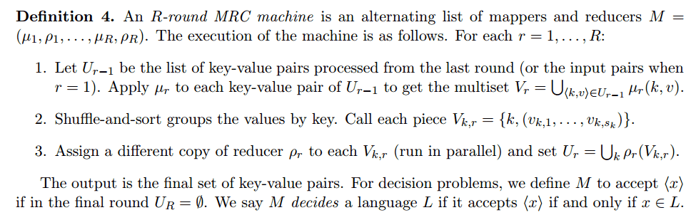
MRC definition
All we’ve done here is just describe the MapReduce protocol in mathematics. It’s messier than it is complicated. The last thing we need is the space bounds.
Definition: A language $ L$ is in $ \textup{MRC}[f(n), g(n)]$ if there is a constant $ 0 < c < 1$ and a sequence of mappers and reducers $ \mu_1, \rho_1, \mu_2, \rho_2, \dots$ such that for all $ x \in \{ 0,1 \}^n$ the following is satisfied:
- Letting $ R = O(f(n))$ and $ M = (\mu_1, \rho_1, \dots, \mu_R, \rho_R)$, $ M$ accepts $ x$ if and only if $ x \in L$.
- For all $ 1 \leq r \leq R$, $ \mu_r, \rho_r$ use $ O(n^c)$ space and $ O(g(n))$ time.
- Each $ \mu_r$ outputs $ O(n^c)$ keys in round $ r$.
To be clear, the first argument to $ \textup{MRC}[f(n), g(n)]$ is the round bound, and the second argument is the time bound. The last point implies the bound on the number of processors. Since we are often interested in a logarithmic number of rounds, we can define
$$\displaystyle \textup{MRC}^i = \textup{MRC}[\log^i(n), \textup{poly}(n)]$$So we can restate the question from the beginning of the post as,
Is graph connectivity in $ \textup{MRC}^0$?
Here there’s a bit of an issue with representation. You have to show that if you’re just given a binary string representing a graph, that you can translate that into a reasonable key-value description of a graph in a constant number of rounds. This is possible, and gives evidence that the key-value representation is without loss of generality for all intents and purposes.
A Pedantic Aside
If our goal is to compare MRC with classes like polynomial time (P) and logarithmic space (L), then the definition above has a problem. Specifically the definition above allows one to have an infinite list of reducers, where each one is potentially different, and the actual machine that is used depends on the input size. In formal terminology, MRC as defined above is a nonuniform model of computation.
Indeed, we give a simple proof that this is a problem by showing any unary language is in $ \textup{MRC}^1$ (which is where many of the MRC algorithms in recent years have been). For those who don’t know, this is a problem because you can encode versions of the Halting problem as a unary language, and the Halting problem is undecidable. We don’t want our model to be able to solve undecidable problems!
While this level of pedantry might induce some eye-rolling, it is necessary in order to make statements like “MRC is contained in P.” It’s simply not true for the nonuniform model above. To fix this problem we refined the MRC model to a uniform version. The details are not trivial, but also not that interesting. Check out the paper if you want to know exactly how we do it. It doesn’t have that much of an effect on the resulting analysis. The only important detail is that now we’re representing the entire MRC machine as a single Turing machine. So now, unlike before, any MRC machine can be written down as a finite string, and there are infinitely many strings representing a specific MRC machine. We call our model MRC, and Karloff’s model nonuniform MRC.
You can also make randomized versions of MRC, but we’ll stick to the deterministic version here.
Sublogarithmic Space
Now we can sketch the proof that sublogarithmic space is in $ \textup{MRC}^0$. In fact, the proof is simpler for regular languages (equivalent to constant space algorithms) being in $ \textup{MRC}^0$. The idea is as follows:
A regular language is one that can be decided by a DFA, say $ G$ (a graph representing state transitions as you read a stream of bits). And the DFA is independent of the input size, so every mapper and reducer can have it encoded into them. Now what we’ll do is split the input string up in contiguous chunks of size $ O(\sqrt{n})$ among the processors (mappers can do this just fine). Now comes the trick. We have each reducer compute, for each possible state $ s$ in $ G$, what the ending state would be if the DFA had started in state $ s$ after processing their chunk of the input. So the output of reducer $ j$ would be an encoding of a table of the form:
$$\displaystyle s_1 \to T_j(s_1) \\\ s_2 \to T_j(s_2) \\\ \vdots \\\ s_{|S|} \to T_j(s_{|S|})$$And the result would be a lookup table of intermediate computation results. So each reducer outputs their part of the table (which has constant size). Since there are only $ O(\sqrt{n})$ reducers, all of the table pieces can fit on a single reducer in the second round, and this reducer can just chain the functions together from the starting state and output the answer.
The proof for sublogarithmic space has the same structure, but is a bit more complicated because one has to account for the tape of a Turing machine which has size $ o(\log n)$. In this case, you split up the tape of the Turing machine among the processors as well. And then you have to keep track of a lot more information. In particular, each entry of your function has to look like
“if my current state is A and my tape contents are B and the tape head starts on side C of my chunk of the input”
then
“the next time the tape head would leave my chunk, it will do so on side C’ and my state will be A’ and my tape contents will be B’.”
As complicated as it sounds, the size of one of these tables for one reducer is still less than $ n^c$ for some $ c < 1/2$. And so we can do the same trick of chaining the functions together to get the final answer. Note that this time the chaining will be adaptive, because whether the tape head leaves the left or right side will determine which part of the table you look at next. And moreover, we know the chaining process will stop in polynomial time because we can always pick a Turing machine to begin with that will halt in polynomial time (i.e., we know that L is contained in P).
The size calculations are also just large enough to stop us from doing the same trick with logarithmic space. So that gives the obvious question: is $ \textup{L} \subset \textup{MRC}^0$? The second part of our paper shows that even weaker containments are probably very hard to prove, and they relate questions about MRC to the problem of L vs P.
Hierarchy Theorems
This part of the paper is where we go much deeper into complexity theory than I imagine most of my readers are comfortable with. Our main theorem looks like this:
Theorem: Assume some conjecture is true. Then for every $ a, b > 0$, there is are bigger $ c > a, d > b$ such that the following hold:
$$ \textup{MRC}[n^a, n^b] \subsetneq \textup{MRC}[n^c, n^b],$$ $$ \textup{MRC}[n^a, n^b] \subsetneq \textup{MRC}[n^a, n^d].$$This is a kind of hierarchy theorem that one often likes to prove in complexity theory. It says that if you give MRC enough extra rounds or time, then you’ll get strictly more computational power.
The conjecture we depend on is called the exponential time hypothesis (ETH), and it says that the 3-SAT problem can’t be solved in $ 2^{cn}$ time for any $ 0 < c < 1$. Actually, our theorem depends on a weaker conjecture (implied by ETH), but it’s easier to understand our theorems in the context of the ETH. Because 3-SAT is this interesting problem: we believe it’s time-intensive, and yet it’s space efficient because we can solve it in linear space given $ 2^n$ time. This time/space tradeoff is one of the oldest questions in all of computer science, but we still don’t have a lot of answers.
For instance, define $ \textup{TISP}(f(n), g(n))$ to the the class of languages that can be decided by Turing machines that have simultaneous bounds of $ O(f(n))$ time and $ O(g(n))$ space. For example, we just said that $ \textup{3-SAT} \in \textup{TISP}(2^n, n)$, and there is a famous theorem that says that SAT is not in $ \textup{TISP}(n^{1.1} n^{0.1})$; apparently this is the best we know. So clearly there are some very basic unsolved problems about TISP. An important one that we address in our paper is whether there are hierarchies in TISP for a fixed amount of space. This is the key ingredient in proving our hierarchy theorem for MRC. In particular here is an open problem:
Conjecture: For every two integers $ 0 < a < b$, the classes $ \textup{TISP}(n^a, n)$ and $ \textup{TISP}(n^b, n)$ are different.
We know this is true of time and space separately, i.e., that $ \textup{TIME}(n^a) \subsetneq \textup{TIME}(n^b)$ and $ \textup{SPACE}(n^a) \subsetneq \textup{SPACE}(n^b)$. but for TISP we only know that you get more power if you increase both parameters.
So we prove a theorem that address this, but falls short in two respects: it depends on a conjecture like ETH, and it’s not for every $ a, b$.
Theorem: Suppose ETH holds, then for every $ a > 0$ there is a $ b > a$ for which $ \textup{TIME}(n^a) \not \subset \textup{TISP}(n^b, n)$.
In words, this suggests that there are problems that need both $ n^2$ time and $ n^2$ space, but can be solved with linear space if you allow enough extra time. Since $ \textup{TISP}(n^a, n) \subset \textup{TIME}(n^a)$, this gives us the hierarchy we wanted.
To prove this we take 3-SAT and give it exponential padding so that it becomes easy enough to do in polynomial TISP (and it still takes linear space, in fact sublinear), but not so easy that you can do it in $ n^a$ time. It takes some more work to get from this TISP hierarchy to our MRC hierarchy, but the details are a bit much for this blog. One thing I’d like to point out is that we prove that statements that are just about MRC have implications beyond MapReduce. In particular, the last corollary of our paper is the following.
Corollary: If $ \textup{MRC}[\textup{poly}(n), 1] \subsetneq \textup{MRC}[\textup{poly}(n), \textup{poly}(n)]$, then L is different from P.
In other words, if you’re afforded a polynomial number of rounds in MRC, then showing that constant time per round is weaker than polynomial time is equivalently hard to separating L from P. The theorem is true because, as it turns out, $ \textup{L} \subset \textup{MRC}[textup{poly}(n), 1]$, by simulating one step of a TM across polynomially many rounds. The proof is actually not that complicated (and doesn’t depend on ETH at all), and it’s a nice demonstration that studying MRC can have implications beyond parallel computing.
The other side of the coin is also interesting. Our first theorem implies the natural question of whether $ \textup{L} \subset \textup{MRC}^0$. We’d like to say that this would imply the separation of L from P, but we don’t quite get that. In particular, we know that
$$\displaystyle \textup{MRC}[1, n] \subsetneq \textup{MRC}[n, n] \subset \textup{MRC}[1, n^2] \subsetneq \textup{MRC}[n^2, n^2] \subset \dots$$But at the same time we could live in a world where
$$\displaystyle \textup{MRC}[1, \textup{poly}(n)] = \textup{MRC}[\textup{poly}(n), \textup{poly}(n)]$$It seems highly unlikely, but to the best of our knowledge none of our techniques prove this is not the case. If we could rule this out, then we could say that $ \textup{L} \subset \textup{MRC}^0$ implies the separation of L and P. And note this would not depend on any conjectures.
Open Problems
Our paper has a list of open problems at the end. My favorite is essentially: how do we prove better lower bounds in MRC? In particular, it would be great if we could show that some problems need a lot of rounds simply because the communication model is too restrictive, and nobody has true random access to the entire input. For example, this is why we think graph connectivity needs a logarithmic number of rounds. But as of now nobody really knows how to prove it, and it seems like we’ll need some new and novel techniques in order to do it. I only have the wisps of ideas in that regard, and it will be fun to see which ones pan out.
Until next time!
Want to respond? Send me an email, post a webmention, or find me elsewhere on the internet.