Linear Programming and the Simplex Algorithm

In the last post in this series we saw some simple examples of linear programs, derived the concept of a dual linear program, and saw the duality theorem and the complementary slackness conditions which give a rough sketch of the stopping criterion for an algorithm. This time we’ll go ahead and write this algorithm for solving linear programs, and next time we’ll apply the algorithm to an industry-strength version of the nutrition problem we saw last time. The algorithm we’ll implement is called the simplex algorithm. It was the first algorithm for solving linear programs, invented in the 1940’s by George Dantzig, and it’s still the leading practical algorithm, and it was a key part of a Nobel Prize. It’s by far one of the most important algorithms ever devised.

As usual, we’ll post all of the code written in the making of this post on this blog’s Github page.

Slack variables and equality constraints

The simplex algorithm can solve any kind of linear program, but it only accepts a special form of the program as input. So first we have to do some manipulations. Recall that the primal form of a linear program was the following minimization problem.

$\min \left \langle c, x \right \rangle \\ \textup{s.t. } Ax \geq b, x \geq 0$

where the brackets mean “dot product.” And its dual is

$\max \left \langle y, b \right \rangle \\ \textup{s.t. } A^Ty \leq c, y \geq 0$

The linear program can actually have more complicated constraints than just the ones above. In general, one might want to have “greater than” and “less than” constraints in the same problem. It turns out that this isn’t any harder, and moreover the simplex algorithm only uses equality constraints, and with some finicky algebra we can turn any set of inequality or equality constraints into a set of equality constraints.

We’ll call our goal the “standard form,” which is as follows:

$\max \left \langle c, x \right \rangle \\ \textup{s.t. } Ax = b, x \geq 0$

It seems impossible to get the usual minimization/maximization problem into standard form until you realize there’s nothing stopping you from adding more variables to the problem. That is, say we’re given a constraint like:

$\displaystyle x_7 + x_3 \leq 10,$

we can add a new variable $\xi$ , called a slack variable, so that we get an equality:

$\displaystyle x_7 + x_3 + \xi = 10$

And now we can just impose that $\xi \geq 0$ . The idea is that $\xi$ represents how much “slack” there is in the inequality, and you can always choose it to make the condition an equality. So if the equality holds and the variables are nonnegative, then the $x_i$ will still satisfy their original inequality. For “greater than” constraints, we can do the same thing but subtract a nonnegative variable. Finally, if we have a minimization problem “ $\min z$ ” we can convert it to $\max -z$ .

So, to combine all of this together, if we have the following linear program with each kind of constraint,

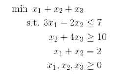
We can add new variables $\xi_1, \xi_2$ , and write it as

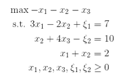
By defining the vector variable $x = (x_1, x_2, x_3, \xi_1, \xi_2)$ and $c = (-1,-1,-1,0,0)$ and $A$ to have $-1, 0, 1$ as appropriately for the new variables, we see that the system is written in standard form.

This is the kind of tedious transformation we can automate with a program. Assuming there are $n$ variables, the input consists of the vector $c$ of length $n$ , and three matrix-vector pairs $(A, b)$ representing the three kinds of constraints. It’s a bit annoying to describe, but the essential idea is that we compute a rectangular “identity” matrix whose diagonal entries are $\pm 1$ , and then join this with the original constraint matrix row-wise. The reader can see the full implementation in the Github repository for this post, though we won’t use this particular functionality in the algorithm that follows.

There are some other additional things we could do: for example there might be some variables that are completely unrestricted. What you do in this case is take an unrestricted variable $z$ and replace it by the difference of two unrestricted variables $z' - z''$ . For simplicity we’ll ignore this, but it would be a fruitful exercise for the reader to augment the function to account for these.

What happened to the slackness conditions?

The “standard form” of our linear program raises an obvious question: how can the complementary slackness conditions make sense if everything is an equality? It turns out that one can redo all the work one did for linear programs of the form we gave last time (minimize w.r.t. greater-than constraints) for programs in the new “standard form” above. We even get the same complementary slackness conditions! If you want to, you can do this entire routine quite a bit faster if you invoke the power of Lagrangians. We won’t do that here, but the tool shows up as a way to work with primal-dual conversions in many other parts of mathematics, so it’s a good buzzword to keep in mind.

In our case, the only difference with the complementary slackness conditions is that one of the two is trivial: $\left \langle y^*, Ax^* - b \right \rangle = 0$ . This is because if our candidate solution $x^*$ is feasible, then it will have to satisfy $Ax = b$ already. The other one, that $\left \langle x^*, A^Ty^* - c \right \rangle = 0$ , is the only one we need to worry about.

Again, the complementary slackness conditions give us inspiration here. Recall that, informally, they say that when a variable is used at all, it is used as much as it can be to fulfill its constraint (the corresponding dual constraint is tight). So a solution will correspond to a choice of some variables which are either used or not, and a choice of nonzero variables will correspond to a solution. We even saw this happen in the last post when we observed that broccoli trumps oranges. If we can get a good handle on how to navigate the set of these solutions, then we’ll have a nifty algorithm.

Let’s make this official and lay out our assumptions.

Extreme points and basic solutions

Remember that the graphical way to solve a linear program is to look at the line (or hyperplane) given by $\langle c, x \rangle = q$ and keep increasing $q$ (or decreasing it, if you are minimizing) until the very last moment when this line touches the region of feasible solutions. Also recall that the “feasible region” is just the set of all solutions to $Ax = b$ , that is the solutions that satisfy the constraints. We imagined this picture:

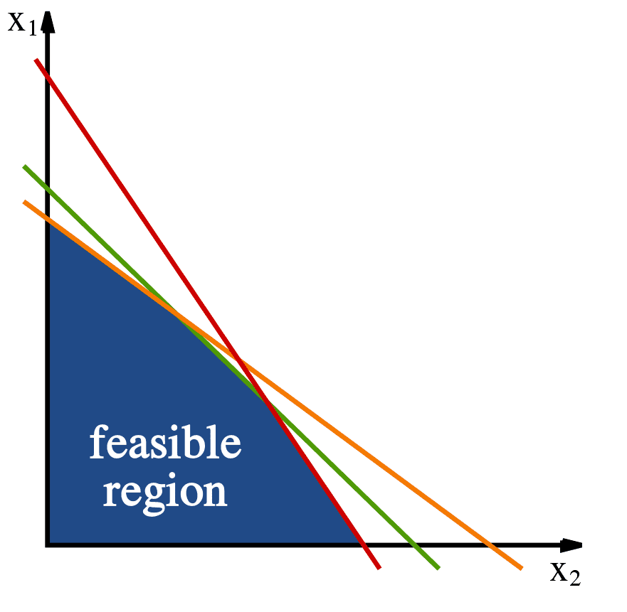
The constraints define a convex area of “feasible solutions.” Image source: Wikipedia.

With this geometric intuition it’s clear that there will always be an optimal solution on a vertex of the feasible region. These points are called extreme points of the feasible region. But because we will almost never work in the plane again (even introducing slack variables makes us relatively high dimensional!) we want an algebraic characterization of these extreme points.

If you have a little bit of practice with convex sets the correct definition is very natural. Recall that a set $X$ is convex if for any two points $x, y \in X$ every point on the line segment between $x$ and $y$ is also in $X$ . An algebraic way to say this (thinking of these points now as vectors) is that every point $\delta x + (1-\delta) y \in X$ when $0 \leq \delta \leq 1$ . Now an extreme point is just a point that isn’t on the inside of any such line, i.e. can’t be written this way for $0 < \delta < 1$ . For example,

A convex set with extremal points in red. Image credit Wikipedia.

Another way to say this is that if $z$ is an extreme point then whenever $z$ can be written as $\delta x + (1-\delta) y$ for some $0 < \delta < 1$ , then actually $x=y=z$ . Now since our constraints are all linear (and there are a finite number of them) they won’t define a convex set with weird curves like the one above. This means that there are a finite number of extreme points that just correspond to the intersections of some of the constraints. So there are at most $2^n$ possibilities.

Indeed we want a characterization of extreme points that’s specific to linear programs in standard form, “ $\max \langle c, x \rangle \textup{ s.t. } Ax=b, x \geq 0$ .” And here is one.

Definition: Let $A$ be an $m \times n$ matrix with $n \geq m$ . A solution $x$ to $Ax=b$ is called basic if at most $m$ of its entries are nonzero.

The reason we call it “basic” is because, under some mild assumptions we describe below, a basic solution corresponds to a vector space basis of $\mathbb{R}^m$ . Which basis? The one given by the $m$ columns of $A$ used in the basic solution. We don’t need to talk about bases like this, though, so in the event of a headache just think of the basis as a set $B \subset \{ 1, 2, \dots, n \}$ of size $m$ corresponding to the nonzero entries of the basic solution.

Indeed, what we’re doing here is looking at the matrix $A_B$ formed by taking the columns of $A$ whose indices are in $B$ , and the vector $x_B$ in the same way, and looking at the equation $A_Bx_B = b$ . If all the parts of $x$ that we removed were zero then this will hold if and only if $Ax=b$ . One might worry that $A_B$ is not invertible, so we’ll go ahead and assume it is. In fact, we’ll assume that every set of $m$ columns of $A$ forms a basis and that the rows of $A$ are also linearly independent. This isn’t without loss of generality because if some rows or columns are not linearly independent, we can remove the offending constraints and variables without changing the set of solutions (this is why it’s so nice to work with the standard form).

Moreover, we’ll assume that every basic solution has exactly $m$ nonzero variables. A basic solution which doesn’t satisfy this assumption is called degenerate, and they’ll essentially be special corner cases in the simplex algorithm. Finally, we call a basic solution feasible if (in addition to satisfying $Ax=b$ ) it satisfies $x \geq 0$ . Now that we’ve made all these assumptions it’s easy to see that choosing $m$ nonzero variables uniquely determines a basic feasible solution. Again calling the sub-matrix $A_B$ for a basis $B$ , it’s just $x_B = A_B^{-1}b$ . Now to finish our characterization, we just have to show that under the same assumptions basic feasible solutions are exactly the extremal points of the feasible region.

Proposition: A vector $x$ is a basic feasible solution if and only if it’s an extreme point of the set $\{ x : Ax = b, x \geq 0 \}$ .

Proof. For one direction, suppose you have a basic feasible solution $x$ , and say we write it as $x = \delta y + (1-\delta) z$ for some $0 < \delta < 1$ . We want to show that this implies $y = z$ . Since all of these points are in the feasible region, all of their coordinates are nonnegative. So whenever a coordinate $x_i = 0$ it must be that both $y_i = z_i = 0$ . Since $x$ has exactly $n-m$ zero entries, it must be that $y, z$ both have at least $n-m$ zero entries, and hence $y,z$ are both basic. By our non-degeneracy assumption they both then have exactly $m$ nonzero entries. Let $B$ be the set of the nonzero indices of $x$ . Because $Ay = Az = b$ , we have $A(y-z) = 0$ . Now $y-z$ has all of its nonzero entries in $B$ , and because the columns of $A_B$ are linearly independent, the fact that $A_B(y-z) = 0$ implies $y-z = 0$ .

In the other direction, suppose that you have some extreme point $x$ which is feasible but not basic. In other words, there are more than $m$ nonzero entries of $x$ , and we’ll call the indices $J = \{ j_1, \dots, j_t \}$ where $t > m$ . The columns of $A_J$ are linearly dependent (since they’re $t$ vectors in $\mathbb{R}^m$ ), and so let $\sum_{i=1}^t z_{j_i} A_{j_i}$ be a nontrivial linear combination of the columns of $A$ . Add zeros to make the $z_{j_i}$ into a length $n$ vector $z$ , so that $Az = 0$ . Now

$A(x + \varepsilon z) = A(x - \varepsilon z) = Ax = b$

And if we pick $\varepsilon$ sufficiently small $x \pm \varepsilon z$ will still be nonnegative, because the only entries we’re changing of $x$ are the strictly positive ones. Then $x = \delta (x + \varepsilon z) + (1 - \delta) \varepsilon z$ for $\delta = 1/2$ , but this is very embarrassing for $x$ who was supposed to be an extreme point. $\square$

Now that we know extreme points are the same as basic feasible solutions, we need to show that any linear program that has some solution has a basic feasible solution. This is clear geometrically: any time you have an optimum it has to either lie on a line or at a vertex, and if it lies on a line then you can slide it to a vertex without changing its value. Nevertheless, it is a useful exercise to go through the algebra.

Theorem. Whenever a linear program is feasible and bounded, it has a basic feasible solution.

Proof. Let $x$ be an optimal solution to the LP. If $x$ has at most $m$ nonzero entries then it’s a basic solution and by the non-degeneracy assumption it must have exactly $m$ nonzero entries. In this case there’s nothing to do, so suppose that $x$ has $r > m$ nonzero entries. It can’t be a basic feasible solution, and hence is not an extreme point of the set of feasible solutions (as proved by the last theorem). So write it as $x = \delta y + (1-\delta) z$ for some feasible $y \neq z$ and $0 < \delta < 1$ .

The only thing we know about $x$ is it’s optimal. Let $c$ be the cost vector, and the optimality says that $\langle c,x \rangle \geq \langle c,y \rangle$ , and $\langle c,x \rangle \geq \langle c,z \rangle$ . We claim that in fact these are equal, that $y, z$ are both optimal as well. Indeed, say $y$ were not optimal, then

$\displaystyle \langle c, y \rangle < \langle c,x \rangle = \delta \langle c,y \rangle + (1-\delta) \langle c,z \rangle$

Which can be rearranged to show that $\langle c,y \rangle < \langle c, z \rangle$ . Unfortunately for $x$ , this implies that it was not optimal all along:

$\displaystyle \langle c,x \rangle < \delta \langle c, z \rangle + (1-\delta) \langle c,z \rangle = \langle c,z \rangle$

An identical argument works to show $z$ is optimal, too. Now we claim we can use $y,z$ to get a new solution that has fewer than $r$ nonzero entries. Once we show this we’re done: inductively repeat the argument with the smaller solution until we get down to exactly $m$ nonzero variables. As before we know that $y,z$ must have at least as many zeros as $x$ . If they have more zeros we’re done. And if they have exactly as many zeros we can do the following trick. Write $w = \gamma y + (1- \gamma)z$ for a $\gamma \in \mathbb{R}$ we’ll choose later. Note that no matter the $\gamma$ , $w$ is optimal. Rewriting $w = z + \gamma (y-z)$ , we just have to pick a $\gamma$ that ensures one of the nonzero coefficients of $z$ is zeroed out while maintaining nonnegativity. Indeed, we can just look at the index $i$ which minimizes $z_i / (y-z)_i$ and use $\delta = - z_i / (y-z)_i$ . $\square$ .

So we have an immediate (and inefficient) combinatorial algorithm: enumerate all subsets of size $m$ , compute the corresponding basic feasible solution $x_B = A_B^{-1}b$ , and see which gives the biggest objective value. The problem is that, even if we knew the value of $m$ , this would take time $n^m$ , and it’s not uncommon for $m$ to be in the tens or hundreds (and if we don’t know $m$ the trivial search is exponential).

So we have to be smarter, and this is where the simplex tableau comes in.

The simplex tableau

Now say you have any basis $B$ and any feasible solution $x$ . For now $x$ might not be a basic solution, and even if it is, its basis of nonzero entries might not be the same as $B$ . We can decompose the equation $Ax = b$ into the basis part and the non basis part:

$A_Bx_B + A_{B'} x_{B'} = b$

and solving the equation for $x_B$ gives

$x_B = A^{-1}_B(b - A_{B'} x_{B'})$

It may look like we’re making a wicked abuse of notation here, but both $A_Bx_B$ and $A_{B'}x_{B'}$ are vectors of length $m$ so the dimensions actually do work out. Now our feasible solution $x$ has to satisfy $Ax = b$ , and the entries of $x$ are all nonnegative, so it must be that $x_B \geq 0$ and $x_{B'} \geq 0$ , and by the equality above $A^{-1}_B (b - A_{B'}x_{B'}) \geq 0$ as well. Now let’s write the maximization objective $\langle c, x \rangle$ by expanding it first in terms of the $x_B, x_{B'}$ , and then expanding $x_B$ .

$\displaystyle \begin{aligned} \langle c, x \rangle & = \langle c_B, x_B \rangle + \langle c_{B'}, x_{B'} \rangle \\ & = \langle c_B, A^{-1}_B(b - A_{B'}x_{B'}) \rangle + \langle c_{B'}, x_{B'} \rangle \\ & = \langle c_B, A^{-1}_Bb \rangle + \langle c_{B'} - (A^{-1}_B A_{B'})^T c_B, x_{B'} \rangle \end{aligned}$

If we want to maximize the objective, we can just maximize this last line. There are two cases. In the first, the vector $c_{B'} - (A^{-1}_B A_{B'})^T c_B \leq 0$ and $A_B^{-1}b \geq 0$ . In the above equation, this tells us that making any component of $x_{B'}$ bigger will decrease the overall objective. In other words, $\langle c, x \rangle \leq \langle c_B, A_B^{-1}b \rangle$ . Picking $x = A_B^{-1}b$ (with zeros in the non basis part) meets this bound and hence must be optimal. In other words, no matter what basis $B$ we’ve chosen (i.e., no matter the candidate basic feasible solution), if the two conditions hold then we’re done.

Now the crux of the algorithm is the second case: if the conditions aren’t met, we can pick a positive index of $c_{B'} - (A_B^{-1}A_{B'})^Tc_B$ and increase the corresponding value of $x_{B'}$ to increase the objective value. As we do this, other variables in the solution will change as well (by decreasing), and we have to stop when one of them hits zero. In doing so, this changes the basis by removing one index and adding another. In reality, we’ll figure out how much to increase ahead of time, and the change will correspond to a single elementary row-operation in a matrix.

Indeed, the matrix we’ll use to represent all of this data is called a tableau in the literature. The columns of the tableau will correspond to variables, and the rows to constraints. The last row of the tableau will maintain a candidate solution $y$ to the dual problem. Here’s a rough picture to keep the different parts clear while we go through the details.

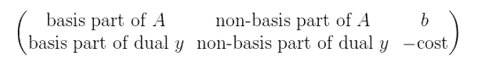
But to make it work we do a slick trick, which is to “left-multiply everything” by $A_B^{-1}$ . In particular, if we have an LP given by $c, A, b$ , then for any basis it’s equivalent to the LP given by $c, A_B^{-1}A, A_{B}^{-1} b$ (just multiply your solution to the new program by $A_B$ to get a solution to the old one). And so the actual tableau will be of this form.

When we say it’s in this form, it’s really only true up to rearranging columns. This is because the chosen basis will always be represented by an identity matrix (as it is to start with), so to find the basis you can find the embedded identity sub-matrix. In fact, the beginning of the simplex algorithm will have the initial basis sitting in the last few columns of the tableau.

Let’s look a little bit closer at the last row. The first portion is zero because $A_B^{-1}A_B$ is the identity. But furthermore with this $A_B^{-1}$ trick the dual LP involves $A_B^{-1}$ everywhere there’s a variable. In particular, joining all but the last column of the last row of the tableau, we have the vector $c - A_B^T(A_B^{-1})^T c$ , and setting $y = A_B^{-1}c_B$ we get a candidate solution for the dual. What makes the trick even slicker is that $A_B^{-1}b$ is already the candidate solution $x_B$ , since $(A_B^{-1}A)_B^{-1}$ is the identity. So we’re implicitly keeping track of two solutions here, one for the primal LP, given by the last column of the tableau, and one for the dual, contained in the last row of the tableau.

I told you the last row was the dual solution, so why all the other crap there? This is the final slick in the trick: the last row further encodes the complementary slackness conditions. Now that we recognize the dual candidate sitting there, the complementary slackness conditions simply ask for the last row to be non-positive (this is just another way of saying what we said at the beginning of this section!). You should check this, but it gives us a stopping criterion: if the last row is non-positive then stop and output the last column.

The simplex algorithm

Now (finally!) we can describe and implement the simplex algorithm in its full glory. Recall that our informal setup has been:

Find an initial basic feasible solution, and set up the corresponding tableau.
Find a positive index of the last row, and increase the corresponding variable (adding it to the basis) just enough to make another variable from the basis zero (removing it from the basis).
Repeat step 2 until the last row is nonpositive.
Output the last column.

This is almost correct, except for some details about how increasing the corresponding variables works. What we’ll really do is represent the basis variables as pivots (ones in the tableau) and then the first 1 in each row will be the variable whose value is given by the entry in the last column of that row. So, for example, the last entry in the first row may be the optimal value for $x_5$ , if the fifth column is the first entry in row 1 to have a 1.

As we describe the algorithm, we’ll illustrate it running on a simple example. In doing this we’ll see what all the different parts of the tableau correspond to from the previous section in each step of the algorithm.

Spoiler alert: the optimum is $x_1 = 2, x_2 = 1$ and the value of the max is 8.

So let’s be more programmatically formal about this. The main routine is essentially pseudocode, and the difficulty is in implementing the helper functions

def simplex(c, A, b):
   tableau = initialTableau(c, A, b)

   while canImprove(tableau):
      pivot = findPivotIndex(tableau)
      pivotAbout(tableau, pivot)

   return primalSolution(tableau), objectiveValue(tableau)

Let’s start with the initial tableau. We’ll assume the user’s inputs already include the slack variables. In particular, our example data before adding slack is

c = [3, 2]
A = [[1, 2], [1, -1]]
b = [4, 1]

And after adding slack:

c = [3, 2, 0, 0]
A = [[1,  2,  1,  0],
     [1, -1,  0,  1]]
b = [4, 1]

Now to set up the initial tableau we need an initial feasible solution in mind. The reader is recommended to work this part out with a pencil, since it’s much easier to write down than it is to explain. Since we introduced slack variables, our initial feasible solution (basis) $B$ can just be $(0,0,1,1)$ . And so $x_B$ is just the slack variables, $c_B$ is the zero vector, and $A_B$ is the 2×2 identity matrix. Now $A_B^{-1}A_{B'} = A_{B'}$ , which is just the original two columns of $A$ we started with, and $A_B^{-1}b = b$ . For the last row, $c_B$ is zero so the part under $A_B^{-1}A_B$ is the zero vector. The part under $A_B^{-1}A_{B'}$ is just $c_{B'} = (3,2)$ .

Rather than move columns around every time the basis $B$ changes, we’ll keep the tableau columns in order of $(x_1, \dots, x_n, \xi_1, \dots, \xi_m)$ . In other words, for our example the initial tableau should look like this.

[[ 1,  2,  1,  0,  4],
 [ 1, -1,  0,  1,  1],
 [ 3,  2,  0,  0,  0]]

So implementing initialTableau is just a matter of putting the data in the right place.

def initialTableau(c, A, b):
   tableau = [row[:] + [x] for row, x in zip(A, b)]
   tableau.append(c[:] + [0])
   return tableau

As an aside: in the event that we don’t start with the trivial basic feasible solution of “trivially use the slack variables,” we’d have to do a lot more work in this function. Next, the primalSolution() and objectiveValue() functions are simple, because they just extract the encoded information out from the tableau (some helper functions are omitted for brevity).

def primalSolution(tableau):
   # the pivot columns denote which variables are used
   columns = transpose(tableau)
   indices = [j for j, col in enumerate(columns[:-1]) if isPivotCol(col)]
   return list(zip(indices, columns[-1]))

def objectiveValue(tableau):
   return -(tableau[-1][-1])

Similarly, the canImprove() function just checks if there’s a nonnegative entry in the last row

def canImprove(tableau):
   lastRow = tableau[-1]
   return any(x > 0 for x in lastRow[:-1])

Let’s run the first loop of our simplex algorithm. The first step is checking to see if anything can be improved (in our example it can). Then we have to find a pivot entry in the tableau. This part includes some edge-case checking, but if the edge cases aren’t a problem then the strategy is simple: find a positive entry corresponding to some entry $j$ of $B'$ , and then pick an appropriate entry in that column to use as the pivot. Pivoting increases the value of $x_j$ (from zero) to whatever is the largest we can make it without making some other variables become negative. As we’ve said before, we’ll stop increasing $x_j$ when some other variable hits zero, and we can compute which will be the first to do so by looking at the current values of $x_B = A_B^{-1}b$ (in the last column of the tableau), and seeing how pivoting will affect them. If you stare at it for long enough, it becomes clear that the first variable to hit zero will be the entry $x_i$ of the basis for which $x_i / A_{i,j}$ is minimal (and $A_{i,j}$ has to be positve). This is because, in order to maintain the linear equalities, every entry of $x_B$ will be decreased by that value during a pivot, and we can’t let any of the variables become negative.

All of this results in the following function, where we have left out the degeneracy/unboundedness checks.

[UPDATE 2018-04-21]: The pivot choices are not as simple as I thought at the time I wrote this. See the discussion on this issue, but the short story is that I was increasing the variable too much, and to fix it it’s easier to update the pivot column choice to be the smallest positive entry of the last row. The code on github is updated to reflect that, but this post will remain unchanged.

def findPivotIndex(tableau):
   # pick first nonzero index of the last row
   column = [i for i,x in enumerate(tableau[-1][:-1]) if x > 0][0]
   quotients = [(i, r[-1] / r[column]) for i,r in enumerate(tableau[:-1]) if r[column] > 0]

   # pick row index minimizing the quotient
   row = min(quotients, key=lambda x: x[1])[0]
   return row, column

For our example, the minimizer is the $(1,0)$ entry (second row, first column). Pivoting is just doing the usual elementary row operations (we covered this in a primer a while back on row-reduction). The pivot function we use here is no different, and in particular mutates the list in place.

def pivotAbout(tableau, pivot):
   i,j = pivot

   pivotDenom = tableau[i][j]
   tableau[i] = [x / pivotDenom for x in tableau[i]]

   for k,row in enumerate(tableau):
      if k != i:
         pivotRowMultiple = [y * tableau[k][j] for y in tableau[i]]
         tableau[k] = [x - y for x,y in zip(tableau[k], pivotRowMultiple)]

And in our example pivoting around the chosen entry gives the new tableau.

[[ 0.,  3.,  1., -1.,  3.],
 [ 1., -1.,  0.,  1.,  1.],
 [ 0.,  5.,  0., -3., -3.]]

In particular, $B$ is now $(1,0,1,0)$ , since our pivot removed the second slack variable $\xi_2$ from the basis. Currently our solution has $x_1 = 1, \xi_1 = 3$ . Notice how the identity submatrix is still sitting in there, the columns are just swapped around.

There’s still a positive entry in the bottom row, so let’s continue. The next pivot is (0,1), and pivoting around that entry gives the following tableau:

[[ 0.        ,  1.        ,  0.33333333, -0.33333333,  1.        ],
 [ 1.        ,  0.        ,  0.33333333,  0.66666667,  2.        ],
 [ 0.        ,  0.        , -1.66666667, -1.33333333, -8.        ]]

And because all of the entries in the bottom row are negative, we’re done. We read off the solution as we described, so that the first variable is 2 and the second is 1, and the objective value is the opposite of the bottom right entry, 8.

To see all of the source code, including the edge-case-checking we left out of this post, see the Github repository for this post.

Obvious questions and sad answers

An obvious question is: what is the runtime of the simplex algorithm? Is it polynomial in the size of the tableau? Is it even guaranteed to stop at some point? The surprising truth is that nobody knows the answer to all of these questions! Originally (in the 1940’s) the simplex algorithm actually had an exponential runtime in the worst case, though this was not known until 1972. And indeed, to this day while some variations are known to terminate, no variation is known to have polynomial runtime in the worst case. Some of the choices we made in our implementation (for example, picking the first column with a positive entry in the bottom row) have the potential to cycle, i.e., variables leave and enter the basis without changing the objective at all. Doing something like picking a random positive column, or picking the column which will increase the objective value by the largest amount are alternatives. Unfortunately, every single pivot-picking rule is known to give rise to exponential-time simplex algorithms in the worst case (in fact, this was discovered as recently as 2011!). So it remains open whether there is a variant of the simplex method that runs in guaranteed polynomial time.

But then, in a stunning turn of events, Leonid Khachiyan proved in the 70’s that in fact linear programs can always be solved in polynomial time, via a completely different algorithm called the ellipsoid method. Following that was a method called the interior point method, which is significantly more efficient. Both of these algorithms generalize to problems that are harder than linear programming as well, so we will probably cover them in the distant future of this blog.

Despite the celebratory nature of these two results, people still use the simplex algorithm for industrial applications of linear programming. The reason is that it’s much faster in practice, and much simpler to implement and experiment with.

The next obvious question has to do with the poignant observation that whole numbers are great. That is, you often want the solution to your problem to involve integers, and not real numbers. But adding the constraint that the variables in a linear program need to be integer valued (even just 0-1 valued!) is NP-complete. This problem is called integer linear programming, or just integer programming (IP). So we can’t hope to solve IP, and rightly so: the reader can verify easily that boolean satisfiability instances can be written as linear programs where each clause corresponds to a constraint.

This brings up a very interesting theoretical issue: if we take an integer program and just remove the integrality constraints, and solve the resulting linear program, how far away are the two solutions? If they’re close, then we can hope to give a good approximation to the integer program by solving the linear program and somehow turning the resulting solution back into an integer solution. In fact this is a very popular technique called LP-rounding. We’ll also likely cover that on this blog at some point.

Oh there’s so much to do and so little time! Until next time.

3 thoughts on “Linear Programming and the Simplex Algorithm”

Paul Coelho

December 18, 2014 at 5:04 pm Reply

To find the cardinality of a certain kind of polytope, I developed what I call sidedness geometry. I believe it might apply to linear programming. In particular, finding a terminating algorithm is trivial, though probably not as optimal as the one you present. Essentially, the problem is to find a region in an n-dimensional space of affine surfaces. In my blog, I present and prove the rules for whether a space and region exist. In short, the algorithm would add boundaries one at a time to a symbolic space in agreement with the numeric surfaces. Then it is a simple matter to answer whether the desired region exists in the symbolic space. In fact using the symbolic space, we can identify which boundaries form the shell of the region. Furthermore, we could find what I call sections wrt the shell boundaries, thus identifying the facets of the desired region. This technique of using a symbolic representation of the affine surfaces may be useful when multiple regions are of interest in the same space.

LikeLike
Murat Aygen

July 3, 2017 at 7:51 am Reply

Remember the familiar ( c_{j} − z_{j} ) coefficients of the zero-row of the Simplex Tableau. Let k(i) be the function returning the index of the Departing Variable when the Pivot in on the i.th row. Then
z_{j} = ∑ c_{k(i)} y_{i, j} where the summation is over i=1, …, m; and y_{i, j}’s are Tableau entries.
Can anybody prove this? I cannot find a numerical counter-example.

LikeLike
Terry

August 22, 2020 at 9:16 am Reply

Hi Jeremy,

Thanks for the great post.

If the geometrical illustration of the problem is “easily” understandable for the primal problem, I struggle to visualize geometrically the backwards and forwards movements between the primal and the dual problem (if I understood correctly the algorithm).

Would you have any material to help visualize the relationship between the two dual problems ?

LikeLike