Quantum mechanics is one of the leading scientific theories describing the rules that govern the universe. It’s discovery and formulation was one of the most important revolutions in the history of mankind, contributing in no small part to the invention of the transistor and the laser.
Here at Math ∩ Programming we don’t put too much emphasis on physics or engineering, so it might seem curious to study quantum physics. But as the reader is likely aware, quantum mechanics forms the basis of one of the most interesting models of computing since the Turing machine: the quantum circuit. My goal with this series is to elucidate the algorithmic insights in quantum algorithms, and explain the mathematical formalisms while minimizing the amount of “interpreting” and “debating” and “experimenting” that dominates so much of the discourse by physicists.
Indeed, the more I learn about quantum computing the more it’s become clear that the shroud of mystery surrounding quantum topics has a lot to do with their presentation. The people teaching quantum (writing the textbooks, giving the lectures, writing the Wikipedia pages) are almost all purely physicists, and they almost unanimously follow the same path of teaching it.
Scott Aaronson (one of the few people who explains quantum in a way I understand) describes the situation superbly.
There are two ways to teach quantum mechanics. The first way – which for most physicists today is still the only way – follows the historical order in which the ideas were discovered. So, you start with classical mechanics and electrodynamics, solving lots of grueling differential equations at every step. Then, you learn about the “blackbody paradox” and various strange experimental results, and the great crisis that these things posed for physics. Next, you learn a complicated patchwork of ideas that physicists invented between 1900 and 1926 to try to make the crisis go away. Then, if you’re lucky, after years of study, you finally get around to the central conceptual point: that nature is described not by probabilities (which are always nonnegative), but by numbers called amplitudes that can be positive, negative, or even complex.
The second way to teach quantum mechanics eschews a blow-by-blow account of its discovery, and instead starts directly from the conceptual core – namely, a certain generalization of the laws of probability to allow minus signs (and more generally, complex numbers). Once you understand that core, you can then sprinkle in physics to taste, and calculate the spectrum of whatever atom you want.
Indeed, the sequence of experiments and debate has historical value. But the mathematics needed to have a basic understanding of quantum mechanics is quite simple, and it is often blurred by physicists in favor of discussing interpretations. To start thinking about quantum mechanics you only need to a healthy dose of linear algebra, and most of it we’ve covered in the three linear algebra primers on this blog. More importantly for computing-minded folks, one only needs a basic understanding of quantum mechanics to understand quantum computing.
The position I want to assume on this blog is that we don’t care about whether quantum mechanics is an accurate description of the real world. The real world gave an invaluable inspiration, but at the end of the day the mathematics stands on its own merits. The really interesting question to me is how the quantum computing model compares to classical computing. Most people believe it is strictly stronger in terms of efficiency. And so the murky depths of the quantum swamp must be hiding some fascinating algorithmic ideas. I want to understand those ideas, and explain them up to my own standards of mathematical rigor and lucidity.
So let’s begin this process with a discussion of an experiment that motivates most of the ideas we’ll need for quantum computing. Hopefully this will be the last experiment we discuss.
Shooting Photons and The Question of Randomness
Does the world around us have inherent randomness in it? This is a deep question open to a lot of philosophical debate, but what evidence do we have that there is randomness?
Here’s the experiment. You set up a contraption that shoots photons in a straight line, aimed at what’s called a “beam splitter.” A beam splitter seems to have the property that when photons are shot at it, they will be either be reflected at a 90 degree angle or stay in a straight line with probability 1/2. Indeed, if you put little photon receptors at the end of each possible route (straight or up, as below) to measure the number of photons that end at each receptor, you’ll find that on average half of the photons went up and half went straight.
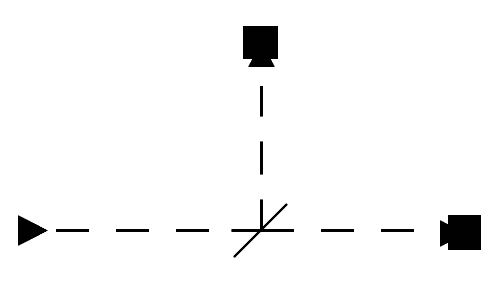
photon-experiment
If you accept that the photon shooter is sufficiently good and the beam splitter is not tricking us somehow, then this is evidence that universe has some inherent randomness in it! Moreover, the probability that a photon goes up or straight seems to be independent of what other photons do, so this is evidence that whatever randomness we’re seeing follows the classical laws of probability. Now let’s augment the experiment as follows. First, put two beam splitters on the corners of a square, and mirrors at the other two corners, as below.
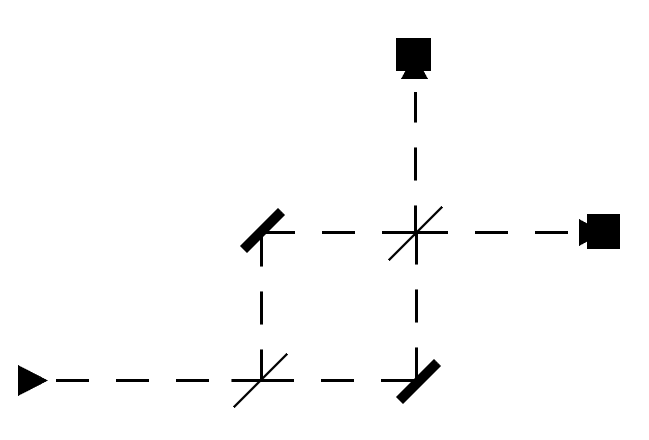
The thicker black lines are mirrors which always reflect the photons.
This is where things get really weird. If you assume that the beam splitter splits photons randomly (as in, according to an independent coin flip), then after the first beam splitter half go up and half go straight, and the same thing would happen after the second beam splitter. So the two receptors should measure half the total number of photons on average.
But that’s not what happens. Rather, all the photons go to the top receptor! Somehow the “probability” that the photon goes left or up in the first beam splitter is connected to the probability that it goes left or up in the second. This seems to be a counterexample to the claim that the universe behaves on the principles of independent probability. Obviously there is some deeper mystery at work.
awardplz
Complex Probabilities
One interesting explanation is that the beam splitter modifies something intrinsic to the photon, something that carries with it until the next beam splitter. You can imagine the photon is carrying information as it shambles along, but regardless of the interpretation it can’t follow the laws of classical probability.
The simplest classical probability explanation would go something like this:
There are two states, RIGHT and UP, and we model the state of a photon by a probability distribution $ (p, q)$ such that the photon has a probability $ p$ of being in state RIGHT a probability $ q$ of being in state UP, and like any probability distribution $ p + q = 1$. A photon hence starts in state $ (1,0)$, and the process of traveling through the beam splitter is the random choice to switch states. This is modeled by multiplication by a particular so-called stochastic matrix (which just means the rows sum to 1)
$$\displaystyle A = \begin{pmatrix} 1/2 & 1/2 \\\ 1/2 & 1/2 \end{pmatrix}$$Of course, we chose this matrix because when we apply it to $ (1,0)$ and $ (0,1)$ we get $ (1/2, 1/2)$ for both outcomes. By doing the algebra, applying it twice to $ (1,0)$ will give the state $ (1/2, 1/2)$, and so the chance of ending up in the top receptor is the same as for the right receptor.
But as we already know this isn’t what happens in real life, so something is amiss. Here is an alternative explanation that gives a nice preview of quantum mechanics.
The idea is that, rather than have the state of the traveling photon be a probability distribution over RIGHT and UP, we have it be a unit vector in a vector space (over $ \mathbb{C}$). That is, now RIGHT and UP are the (basis) unit vectors $ e_1 = (1,0), e_2 = (0,1)$, respectively, and a state $ x$ is a linear combination $ c_1 e_1 + c_2 e_2$, where we require $ \left \| x \right \|^2 = |c_1|^2 + |c_2|^2 = 1$. And now the “probability” that the photon is in the RIGHT state is the square of the coefficient for that basis vector $ p_{\text{right}} = |c_1|^2$. Likewise, the probability of being in the UP state is $ p_{\text{up}} = |c_2|^2$.
This might seem like an innocuous modification—even a pointless one!—but changing the sum (or 1-norm) to the Euclidean sum-of-squares (or the 2-norm) is at the heart of why quantum mechanics is so different. Now rather than have stochastic matrices for state transitions, which are defined they way they are because they preserve probability distributions, we use unitary matrices, which are those complex-valued matrices that preserve the 2-norm. In both cases, we want “valid states” to be transformed into “valid states,” but we just change precisely what we mean by a state, and pick the transformations that preserve that.
In fact, as we’ll see later in this series using complex numbers is totally unnecessary. Everything that can be done with complex numbers can be done without them (up to a good enough approximation for computing), but using complex numbers just happens to make things more elegant mathematically. It’s the kind of situation where there are more and better theorems in linear algebra about complex-valued matrices than real valued matrices.
But back to our experiment. Now we can hypothesize that the beam splitter corresponds to the following transformation of states:
$$\displaystyle A = \frac{1}{\sqrt{2}} \begin{pmatrix} 1 & i \\\ i & 1 \end{pmatrix}$$We’ll talk a lot more about unitary matrices later, so for now the reader can rest assured that this is one. And then how does it transform the initial state $ x =(1,0)$?
$$\displaystyle y = Ax = \frac{1}{\sqrt{2}}(1, i)$$So at this stage the probability of being in the RIGHT state is $ 1/2 = (1/\sqrt{2})^2$ and the probability of being in state UP is also $ 1/2 = |i/\sqrt{2}|^2$. So far it matches the first experiment. Applying $ A$ again,
$$\displaystyle Ay = A^2x = \frac{1}{2}(0, 2i) = (0, i)$$And the photon is in state UP with probability 1. Stunning. This time Science is impressed by mathematics.
Next time we’ll continue this train of thought by generalizing the situation to the appropriate mathematical setting. Then we’ll dive into the quantum circuit model, and start churning out some algorithms.
Until then!
[Edit: Actually, if you make the model complicated enough, then you can achieve the result using classical probability. The experiment I described above, while it does give evidence that something more complicated is going on, it does not fully rule out classical probability. Mathematically, you can lay out the axioms of quantum mechanics (as we will from the perspective of computing), and mathematically this forces non-classical probability. But to the best of my knowledge there is no experiment or set of experiments that gives decisive proof that all of the axioms are necessary. In my search for such an experiment I asked this question on stackexchange and didn’t understand any of the answers well enough to paraphrase them here. Moreover, if you leave out the axiom that quantum circuit operations are reversible, you can do everything with classical probability. I read this somewhere but now I can’t find the source 🙁
One consequence is that I am more firmly entrenched in my view that I only care about quantum mechanics in how it produced quantum computing as a new paradigm in computer science. This paradigm doesn’t need physics at all, and apparently the motivations for the models are still unclear, so we just won’t discuss them any more. Sorry, physics lovers.]
Want to respond? Send me an email, post a webmention, or find me elsewhere on the internet.