There are two basic problems in information theory that are very easy to explain. Two people, Alice and Bob, want to communicate over a digital channel over some long period of time, and they know the probability that certain messages will be sent ahead of time. For example, English language sentences are more likely than gibberish, and “Hi” is much more likely than “asphyxiation.” The problems are:
- Say communication is very expensive. Then the problem is to come up with an encoding scheme for the messages which minimizes the expected length of an encoded message and guarantees the ability to unambiguously decode a message. This is called the noiseless coding problem.
- Say communication is not expensive, but error prone. In particular, each bit $ i$ of your message is erroneously flipped with some known probably $ p$, and all the errors are independent. Then the question is, how can one encode their messages to as to guarantee (with high probability) the ability to decode any sent message? This is called the noisy coding problem.
There are actually many models of “communication with noise” that generalize (2), such as models based on Markov chains. We are not going to cover them here.
Here is a simple example for the noiseless problem. Say you are just sending binary digits as your messages, and you know that the string “00000000” (eight zeros) occurs half the time, and all other eight-bit strings occur equally likely in the other half. It would make sense, then, to encode the “eight zeros” string as a 0, and prefix all other strings with a 1 to distinguish them from zero. You would save on average $ 7 \cdot 1/2 + (-1) \cdot 1/2 = 3$ bits in every message.
One amazing thing about these two problems is that they were posed and solved in the same paper by Claude Shannon in 1948. One byproduct of his work was the notion of entropy, which in this context measures the “information content” of a message, or the expected “compressibility” of a single bit under the best encoding. For the extremely dedicated reader of this blog, note this differs from Kolmogorov complexity in that we’re not analyzing the compressibility of a string by itself, but rather when compared to a distribution. So really we should think of (the domain of) the distribution as being compressed, not the string.

Claude Shannon. Image credit: [Wikipedia](http://en.wikipedia.org/wiki/Claude_Shannon)
Entropy and noiseless encoding
Before we can state Shannon’s theorems we have to define entropy.
Definition: Suppose $ D$ is a distribution on a finite set $ X$, and I’ll use $ D(x)$ to denote the probability of drawing $ x$ from $ D$. The entropy of $ D$, denoted $ H(D)$ is defined as
$$H(D) = \sum_{x \in X} D(x) \log \frac{1}{D(x)}$$It is strange to think about this sum in abstract, so let’s suppose $ D$ is a biased coin flip with bias $ 0 \leq p \leq 1$ of landing heads. Then we can plot the entropy as follows
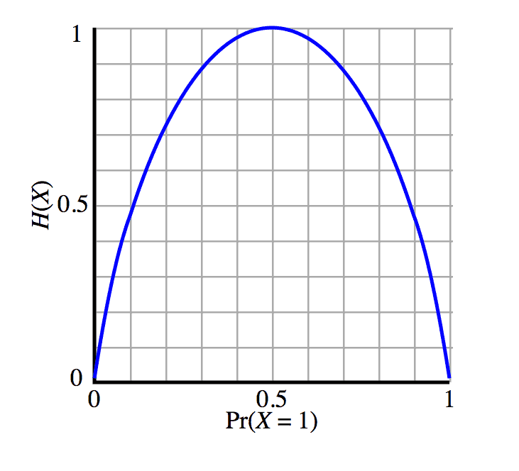
Image source: Wikipedia
The horizontal axis is the bias $ p$, and the vertical axis is the value of $ H(D)$, which with some algebra is $ – p \log p – (1-p) \log (1-p)$. From the graph above we can see that the entropy is maximized when $ p=1/2$ and minimized at $ p=0, 1$. You can verify all of this with calculus, and you can prove that the uniform distribution maximizes entropy in general as well.
So what is this saying? A high entropy measures how incompressible something is, and low entropy gives us lots of compressibility. Indeed, if our message consisted of the results of 10 such coin flips, and $ p$ was close to 1, we could be able to compress a lot by encoding strings with lots of 1’s using few bits. On the other hand, if $ p=1/2$ we couldn’t get any compression at all. All strings would be equally likely.
Shannon’s famous theorem shows that the entropy of the distribution is actually all that matters. Some quick notation: $ \{ 0,1 \}^*$ is the set of all binary strings.
Theorem (Noiseless Coding Theorem) [Shannon 1948]: For every finite set $ X$ and distribution $ D$ over $ X$, there are encoding and decoding functions $ \textup{Enc}: X \to \{0,1 \}^*, \textup{Dec}: \{ 0,1 \}^* \to X$ such that
- The encoding/decoding actually works, i.e. $ \textup{Dec}(\textup{Enc}(x)) = x$ for all $ x$.
- The expected length of an encoded message is between $ H(D)$ and $ H(D) + 1$.
Moreover, no encoding scheme can do better.
Item 2 and the last sentence are the magical parts. In other words, if you know your distribution over messages, you precisely know how long to expect your messages to be. And you know that you can’t hope to do any better!
As the title of this post says, we aren’t going to give a proof here. Wikipedia has a proof if you’re really interested in the details.
Noisy Coding
The noisy coding problem is more interesting because in a certain sense (that was not solved by Shannon) it is still being studied today in the field of coding theory. The interpretation of the noisy coding problem is that you want to be able to recover from white noise errors introduced during transmission. The concept is called error correction. To restate what we said earlier, we want to recover from error with probability asymptotically close to 1, where the probability is over the errors.
It should be intuitively clear that you can’t do so without your encoding “blowing up” the length of the messages. Indeed, if your encoding does not blow up the message length then a single error will confound you since many valid messages would differ by only a single bit. So the question is does such an encoding exist, and if so how much do we need to blow up the message length? Shannon’s second theorem answers both questions.
Theorem (Noisy Coding Theorem) [Shannon 1948]: For any constant noise rate $ p < 1/2$, there is an encoding scheme $ \textup{Enc} : \{ 0,1 \}^k \to \{0,1\}^{ck}, \textup{Dec} : \{ 0,1 \}^{ck} \to \{ 0,1\}^k$ with the following property. If $ x$ is the message sent by Alice, and $ y$ is the message received by Bob (i.e. $ \textup{Enc}(x)$ with random noise), then $ \Pr[\textup{Dec}(y) = x] \to 1$ as a function of $ n=ck$. In addition, if we denote by $ H(p)$ the entropy of the distribution of an error on a single bit, then choosing any $ c > \frac{1}{1-H(p)}$ guarantees the existence of such an encoding scheme, and no scheme exists for any smaller $ c$.
This theorem formalizes a “yes” answer to the noisy coding problem, but moreover it characterizes the blowup needed for such a scheme to exist. The deep fact is that it only depends on the noise rate.
A word about the proof: it’s probabilistic. That is, Shannon proved such an encoding scheme exists by picking $ \textup{Enc}$ to be a random function (!). Then $ \textup{Dec}(y)$ finds (nonconstructively) the string $ x$ such that the number of bits different between $ \textup{Enc}(x)$ and $ y$ is minimized. This “number of bits that differ” measure is called the Hamming distance. Then he showed using relatively standard probability tools that this scheme has the needed properties with high probability, the implication being that some scheme has to exist for such a probability to even be positive. The sharp threshold for $ c$ takes a bit more work. If you want the details, check out the first few lectures of Madhu Sudan’s MIT class.
The non-algorithmic nature of his solution is what opened the door to more research. The question has surpassed, “Are there any encodings that work?” to the more interesting, “What is the algorithmic cost of constructing such an encoding?” It became a question of complexity, not computability. Moreover, the guarantees people wanted were strengthened to worst case guarantees. In other words, if I can guarantee at most 12 errors, is there an encoding scheme that will allow me to always recover the original message, and not just with high probability? One can imagine that if your message contains nuclear codes or your bank balance, you’d definitely want to have 100% recovery ability.
Indeed, two years later Richard Hamming spawned the theory of error correcting codes and defined codes that can always correct a single error. This theory has expanded and grown over the last sixty years, and these days the algorithmic problems of coding theory have deep connections to most areas of computer science, including learning theory, cryptography, and quantum computing.
We’ll cover Hamming’s basic codes next time, and then move on to Reed-Solomon codes and others. Until then!
Posts in this series:
- A Proofless Introduction to Coding Theory
- Hamming’s Code
- The Codes of Solomon, Reed, and Muller
- The Welch-Berlekamp Algorithm for Correcting Errors in Data
Want to respond? Send me an email, post a webmention, or find me elsewhere on the internet.