Hamming's Code

Or how to detect and correct errors

Last time we made a quick tour through the main theorems of Claude Shannon, which essentially solved the following two problems about communicating over a digital channel.

1. What is the best encoding for information when you are guaranteed that your communication channel is error free?
2. Are there any encoding schemes that can recover from random noise introduced during transmission?

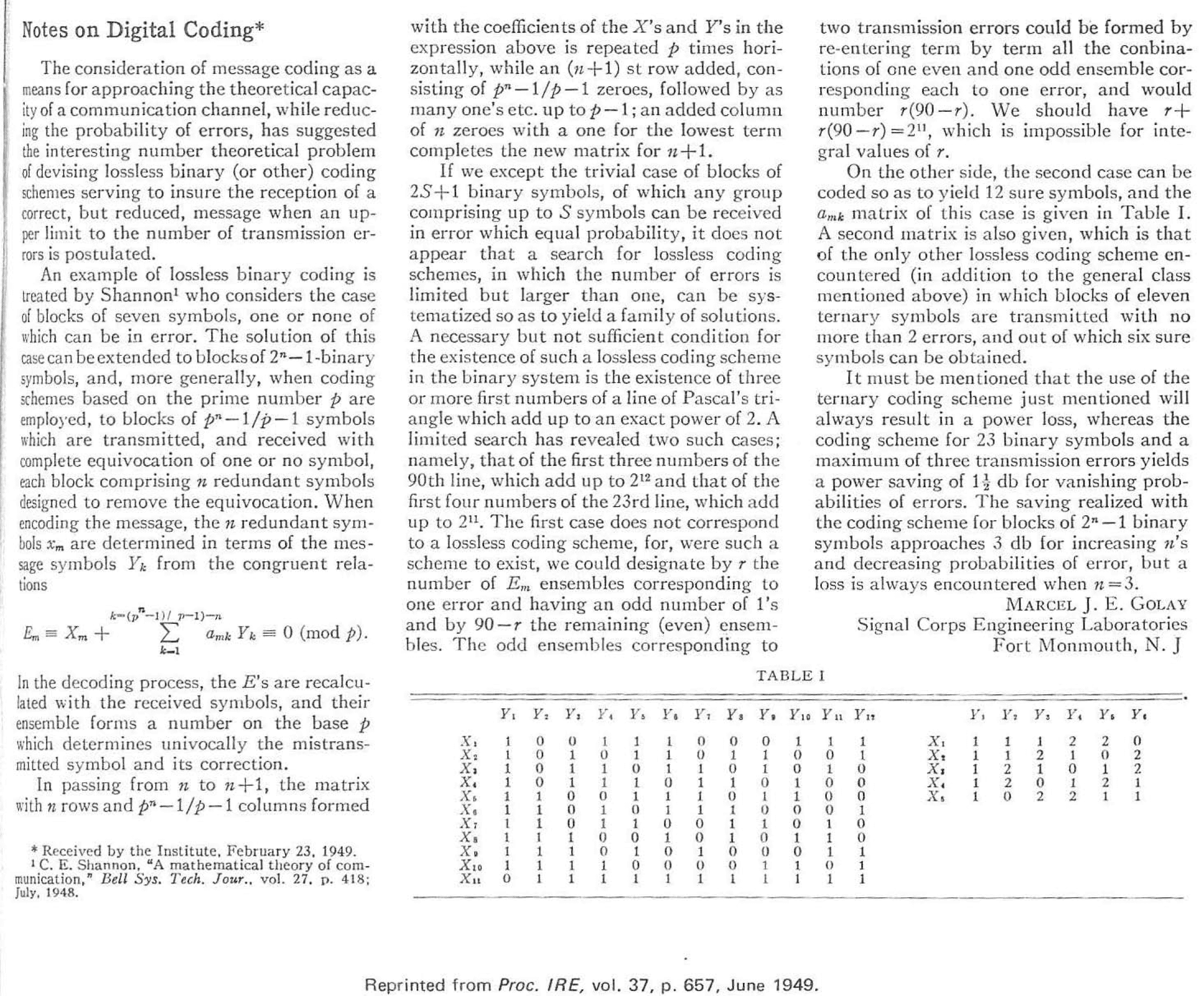
The answers to these questions were purely mathematical theorems, of course. But the interesting shortcoming of Shannon’s accomplishment was that his solution for the noisy coding problem (2) was nonconstructive. The question remains: can we actually come up with efficiently computable encoding schemes? The answer is yes! Marcel Golay was the first to discover such a code in 1949 (just a year after Shannon’s landmark paper), and Golay’s construction was published on a single page! We’re not going to define Golay’s code in this post, but we will mention its interesting status in coding theory later. The next year Richard Hamming discovered another simpler and larger family of codes, and went on to do some of the major founding work in coding theory. For his efforts he won a Turing Award and played a major part in bringing about the modern digital age. So we’ll start with Hamming’s codes.

We will assume some basic linear algebra knowledge, as detailed our first linear algebra primer. We will also use some basic facts about polynomials and finite fields, though the lazy reader can just imagine everything as binary $\{0,1\}$ and still grok the important stuff.

What is a code?

The formal definition of a code is simple: a code $C$ is just a subset of $\{0,1{\}}^n$ for some $n$. Elements of $C$ are called codewords.

This is deceptively simple, but here’s the intuition. Say we know we want to send messages of length $k$, so that our messages are in $\{0,1{\}}^k$. Then we’re really viewing a code $C$ as the image of some encoding function $\text{Enc}:\{0,1{\}}^k\to \{0,1{\}}^n$. We can define $C$ by just describing what the set is, or we can define it by describing the encoding function. Either way, we will make sure that $\text{Enc}$ is an injective function, so that no two messages get sent to the same codeword. Then $|C|=2^k$, and we can call $k=\log |C|$ the message length of $C$ even if we don’t have an explicit encoding function.

Moreover, while in this post we’ll always work with $\{0,1\}$, the alphabet of your encoded messages could be an arbitrary set $\mathrm{\Sigma }$. So then a code $C$ would be a subset of tuples in ${\mathrm{\Sigma }}^n$, and we would call $q=|\mathrm{\Sigma }|$.

So we have these parameters $n,k,q$, and we need one more. This is the minimum distance of a code, which we’ll denote by $d$. This is defined to be the minimum Hamming distance between all distinct pairs of codewords, where by Hamming distance I just mean the number of coordinates that two tuples differ in. Recalling the remarks we made last time about Shannon’s nonconstructive proof, when we decode an encoded message $y$ (possibly with noisy bits) we look for the (unencoded) message $x$ whose encoding $\text{Enc}(x)$ is as close to $y$ as possible. This will only work in the worst case if all pairs of codewords are sufficiently far apart. Hence we track the minimum distance of a code.

So coding theorists turn this mess of parameters into notation.

Definition: A code $C$ is called an $(n,k,d{)}_q$-code if

• $C\subset {\mathrm{\Sigma }}^n$ for some alphabet $\mathrm{\Sigma }$,
• $k=\log |C|$,
• $C$ has minimum distance $d$, and
• the alphabet $\mathrm{\Sigma }$ has size $q$.

The basic goals of coding theory are:

1. For which values of these four parameters do codes exist?
2. Fixing any three parameters, how can we optimize the other one?

In this post we’ll see how simple linear-algebraic constructions can give optima for one of these problems, optimizing $k$ for $d=3$, and we’ll state a characterization theorem for optimizing $k$ for a general $d$. Next time we’ll continue with a second construction that optimizes a different bound called the Singleton bound.

Linear codes and the Hamming code

A code is called linear if it can be identified with a linear subspace of some finite-dimensional vector space. In this post all of our vector spaces will be $\{0,1{\}}^n$, that is tuples of bits under addition mod 2. But you can do the same constructions with any finite scalar field ${\mathbb{F}}_q$ for a prime power $q$, i.e. have your vector space be ${\mathbb{F}}_q^n$. We’ll go back and forth between describing a binary code $q=2$ over $\{0,1\}$ and a code in ${\mathbb{F}}_q^n$. So to say a code is linear means:

• The zero vector is a codeword.
• The sum of any two codewords is a codeword.
• Any scalar multiple of a codeword is a codeword.

Linear codes are the simplest kinds of codes, but already they give a rich variety of things to study. The benefit of linear codes is that you can describe them in a lot of different and useful ways besides just describing the encoding function. We’ll use two that we define here. The idea is simple: you can describe everything about a linear subspace by giving a basis for the space.

Definition: A generator matrix of a $(n,k,d{)}_q$-code $C$ is a $k\times n$ matrix $G$ whose rows form a basis for $C$.

There are a lot of equivalent generator matrices for a linear code (we’ll come back to this later), but the main benefit is that having a generator matrix allows one to encode messages $x\in \{0,1{\}}^k$ by left multiplication $xG$. Intuitively, we can think of the bits of $x$ as describing the coefficients of the chosen linear combination of the rows of $G$, which uniquely describes an element of the subspace. Note that because a $k$-dimensional subspace of $\{0,1{\}}^n$ has $2^k$ elements, we’re not abusing notation by calling $k=\log |C|$ both the message length and the dimension.

For the second description of $C$, we’ll remind the reader that every linear subspace $C$ has a unique orthogonal complement $C^{\perp }$, which is the subspace of vectors that are orthogonal to vectors in $C$.

Definition: Let $H^T$ be a generator matrix for $C^{\perp }$. Then $H$ is called a parity check matrix.

Note $H$ has the basis for $C^{\perp }$ as columns. This means it has dimensions $n\times (n-k)$. Moreover, it has the property that $x\in C$ if and only if the left multiplication $xH=0$. Having zero dot product with all columns of $H$ characterizes membership in $C$.

The benefit of having a parity check matrix is that you can do efficient error detection: just compute $yH$ on your received message $y$, and if it’s nonzero there was an error! What if there were so many errors, and just the right errors that $y$ coincided with a different codeword than it started? Then you’re screwed. In other words, the parity check matrix is only guarantee to detect errors if you have fewer errors than the minimum distance of your code.

So that raises an obvious question: if you give me the generator matrix of a linear code can I compute its minimum distance? It turns out that this problem is NP-hard in general. In fact, you can show that this is equivalent to finding the smallest linearly dependent set of rows of the parity check matrix, and it is easier to see why such a problem might be hard. But if you construct your codes cleverly enough you can compute their distance properties with ease.

Before we do that, one more definition and a simple proposition about linear codes. The Hamming weight of a vector $x$, denoted $wt(x)$, is the number of nonzero entries in $x$.

Proposition: The minimum distance of a linear code $C$ is the minimum Hamming weight over all nonzero vectors $x\in C$.

Proof. Consider a nonzero $x\in C$. On one hand, the zero vector is a codeword and $wt(x)$ is by definition the Hamming distance between $x$ and zero, so it is an upper bound on the minimum distance. In fact, it’s also a lower bound: if $x,y$ are two nonzero codewords, then $x-y$ is also a codeword and $wt(x-y)$ is the Hamming distance between $x$ and $y$.

So now we can define our first code, the Hamming code. It will be a $(n,k,3{)}_2$-code. The construction is quite simple. We have fixed $d=3,q=2$, and we will also fix $l=n-k$. One can think of this as fixing $n$ and maximizing $k$, but it will only work for $n$ of a special form.

We’ll construct the Hamming code by describing a parity-check matrix $H$. In fact, we’re going to see what conditions the minimum distance $d=3$ imposes on $H$, and find out those conditions are actually sufficient to get $d=3$. We’ll start with 2. If we want to ensure $d\ge 2$, then you need it to be the case that no nonzero vector of Hamming weight 1 is a code word. Indeed, if $e_i$ is a vector with all zeros except a one in position $i$, then $e_{i}H=h_i$ is the $i$-th row of $H$. We need $e_{i}H\ne 0$, so this imposes the condition that no row of $H$ can be zero. It’s easy to see that this is sufficient for $d\ge 2$.

Likewise for $d\ge 3$, given a vector $y=e_i+e_j$ for some positions $i\ne j$, then $yH=h_i+h_j$ may not be zero. But because our sums are mod 2, saying that $h_i+h_j\ne 0$ is the same as saying $h_i\ne h_j$. Again it’s an if and only if. So we have the two conditions.

• No row of $H$ may be zero.
• All rows of $H$ must be distinct.

That is, any parity check matrix with those two properties defines a distance 3 linear code. The only question that remains is how large can $n$ be if the vectors have length $n-k=l$? That’s just the number of distinct nonzero binary strings of length $l$, which is $2^l–1$. Picking any way to arrange these strings as the rows of a matrix (say, in lexicographic order) gives you a good parity check matrix.

Theorem: For every $l>0$, there is a $(2^l–1,2^l–l–1,3{)}_2$-code called the Hamming code.

Since the Hamming code has distance 3, we can always detect if at most a single error occurs. Moreover, we can correct a single error using the Hamming code. If $x\in C$ and $wt(e)=1$ is an error bit in position $i$, then the incoming message would be $y=x+e$. Now compute $yH=xH+eH=0+eH=h_i$ and flip bit $i$ of $y$. That is, whichever row of $H$ you get tells you the index of the error, so you can flip the corresponding bit and correct it. If you order the rows lexicographically like we said, then $h_i=i$ as a binary number. Very slick.

Before we move on, we should note one interesting feature of linear codes.

Definition: A code is called systematic if it can be realized by an encoding function that appends some number $n-k$ “check bits” to the end of each message.

The interesting feature is that all linear codes are systematic. The reason is as follows. The generator matrix $G$ of a linear code has as rows a basis for the code as a linear subspace. We can perform Gaussian elimination on $G$ and get a new generator matrix that looks like $[I\mid A]$ where $I$ is the identity matrix of the appropriate size and $A$ is some junk. The point is that encoding using this generator matrix leaves the message unchanged, and adds a bunch of bits to the end that are determined by $A$. It’s a different encoding function on $\{0,1{\}}^k$, but it has the same image in $\{0,1{\}}^n$, i.e. the code is unchanged. Gaussian elimination just performed a change of basis.

If you work out the parameters of the Hamming code, you’ll see that it is a systematic code which adds $\mathrm{\Theta }(\log n)$ check bits to a message, and we’re able to correct a single error in this code. An obvious question is whether this is necessary? Could we get away with adding fewer check bits? The answer is no, and a simple “information theoretic” argument shows this. A single index out of $n$ requires $\log n$ bits to describe, and being able to correct a single error is like identifying a unique index. Without logarithmically many bits, you just don’t have enough information.

The Hamming bound and perfect codes

One nice fact about Hamming codes is that they optimize a natural problem: the problem of maximizing $d$ given a fixed choice of $n$, $k$, and $q$. To get this let’s define $V_n(r)$ denote the volume of a ball of radius $r$ in the space ${\mathbb{F}}_2^n$. I.e., if you fix any string (doesn’t matter which) $x$, $V_n(r)$ is the size of the set $\{y:d(x,y)\le r\}$, where $d(x,y)$ is the hamming distance.

There is a theorem called the Hamming bound, which describes a limit to how much you can pack disjoint balls of radius $r$ inside ${\mathbb{F}}_2^n$.

Theorem: If an $(n,k,d{)}_2$-code exists, then

Proof. The proof is quite simple. To say a code $C$ has distance $d$ means that for every string $x\in C$ there is no other string $y$ within Hamming distance $d$ of $x$. In other words, the balls centered around both $x,y$ of radius $r=\lfloor (d-1)/2\rfloor$ are disjoint. The extra difference of one is for odd $d$, e.g. when $d=3$ you need balls of radius 1 to guarantee no overlap. Now $|C|=2^k$, so the total number of strings covered by all these balls is the left-hand side of the expression. But there are at most $2^n$ strings in ${\mathbb{F}}_2^n$, establishing the desired inequality.

Now a code is called perfect if it actually meets the Hamming bound exactly. As you probably guessed, the Hamming codes are perfect codes. It’s not hard to prove this, and I’m leaving it as an exercise to the reader.

The obvious follow-up question is whether there are any other perfect codes. The answer is yes, some of which are nonlinear. But some of them are “trivial.” For example, when $d=1$ you can just use the identity encoding to get the code $C={\mathbb{F}}_2^n$. You can also just have a code which consists of a single codeword. There are also some codes that encode by repeating the message multiple times. These are called “repetition codes,” and all three of these examples are called trivial (as a definition). Now there are some nontrivial and nonlinear perfect codes I won’t describe here, but here is the nice characterization theorem.

Theorem [van Lint ’71, Tietavainen ‘73]: Let $C$ be a nontrivial perfect $(n,d,k{)}_q$ code. Then the parameters must either be that of a Hamming code, or one of the two:

• A $(23,12,7{)}_2$-code
• A $(11,6,5{)}_3$-code

The last two examples are known as the binary and ternary Golay codes, respectively, which are also linear. In other words, every possible set of parameters for a perfect code can be realized as one of these three linear codes.

So this theorem was a big deal in coding theory. The Hamming and Golay codes were both discovered within a year of each other, in 1949 and 1950, but the nonexistence of other perfect linear codes was open for twenty more years. This wrapped up a very neat package.

Next time we’ll discuss the Singleton bound, which optimizes for a different quantity and is incomparable with perfect codes. We’ll define the Reed-Solomon and show they optimize this bound as well. These codes are particularly famous for being the error correcting codes used in DVDs. We’ll then discuss the algorithmic issues surrounding decoding, and more recent connections to complexity theory.

Until then!

Posts in this series:

• A Proofless Introduction to Coding Theory
• Hamming’s Code
• The Codes of Solomon, Reed, and Muller
• The Welch-Berlekamp Algorithm for Correcting Errors in Data