It’s about time we got back to computational topology. Previously in this series we endured a lightning tour of the fundamental group and homology, then we saw how to compute the homology of a simplicial complex using linear algebra.
What we really want to do is talk about the inherent shape of data. Homology allows us to compute some qualitative features of a given shape, i.e., find and count the number of connected components or a given shape, or the number of “2-dimensional holes” it has. This is great, but data doesn’t come in a form suitable for computing homology. Though they may have originated from some underlying process that follows nice rules, data points are just floating around in space with no obvious connection between them.
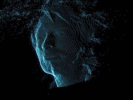
Here is a cool example of Thom Yorke, the lead singer of the band Radiohead, whose face was scanned with a laser scanner for their music video “House of Cards.”
radiohead-still
Given a point cloud such as the one above, our long term goal (we’re just getting started in this post) is to algorithmically discover what the characteristic topological features are in the data. Since homology is pretty coarse, we might detect the fact that the point cloud above looks like a hollow sphere with some holes in it corresponding to nostrils, ears, and the like. The hope is that if the data set isn’t too corrupted by noise, then it’s a good approximation to the underlying space it is sampled from. By computing the topological features of a point cloud we can understand the process that generated it, and Science can proceed.
But it’s not always as simple as Thom Yorke’s face. It turns out the producers of the music video had to actually degrade the data to get what you see above, because their lasers were too precise and didn’t look artistic enough! But you can imagine that if your laser is mounted on a car on a bumpy road, or tracking some object in the sky, or your data comes from acoustic waves traveling through earth, you’re bound to get noise. Or more realistically, if your data comes from thousands of stock market prices then the process generating the data is super mysterious. It changes over time, it may not follow any discernible pattern (though speculators may hope it does), and you can’t hope to visualize the entire dataset in any useful way.
But with persistent homology, so the claim goes, you’d get a good qualitative understanding of the dataset. Your results would be resistant to noise inherent in the data. It also wouldn’t be sensitive to the details of your data cleaning process. And with a dash of ingenuity, you can come up with a reasonable mathematical model of the underlying generative process. You could use that model to design algorithms, make big bucks, discover new drugs, recognize pictures of cats, or whatever tickles your fancy.
But our first problem is to resolve the input data type error. We want to use homology to describe data, but our data is a point cloud and homology operates on simplicial complexes. In this post we’ll see two ways one can do this, and see how they’re related.
The Čech complex
Let’s start with the Čech complex. Given a point set $ X$ in some metric space and a number $ \varepsilon > 0$, the Čech complex $ C_\varepsilon$ is the simplicial complex whose simplices are formed as follows. For each subset $ S \subset X$ of points, form a $ (\varepsilon/2)$-ball around each point in $ S$, and include $ S$ as a simplex (of dimension $ |S|$) if there is a common point contained in all of the balls in $ S$. This structure obviously satisfies the definition of a simplicial complex: any sub-subset $ S’ \subset S$ of a simplex $ S$ will be also be a simplex. Here is an example of the epsilon balls.
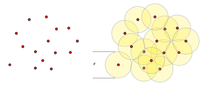
Image credit: Robert Ghrist
Let me superscript the Čech complex to illustrate the pieces. Specifically, we’ll let $ C_\varepsilon^{j}$ denote all the simplices of dimension up to $ j$. In particular, $ C_\varepsilon^1$ is a graph where an edge is placed between $ x,y$ if $ d(x,y) < \varepsilon$, and $ C_{\varepsilon}^2$ places triangles (2-simplices) on triples of points whose balls have a three-way intersection. A topologist will have a minor protest here: the simplicial complex is supposed to resemble the structure inherent in the underlying points, but how do we know that this abstract simplicial complex (which is really hard to visualize!) resembles the topological space we used to make it? That is, $ X$ was sitting in some metric space, and the union of these epsilon-balls forms some topological space $ X(\varepsilon)$ that is close in structure to $ X$. But is the Čech complex $ C_\varepsilon$ close to $ X(\varepsilon)$? Do they have the same topological structure? It’s not a trivial theorem to prove, but it turns out to be true.
The Nerve Theorem: The homotopy types of $ X(\varepsilon)$ and $ C_\varepsilon$ are the same.
We won’t remind the readers about homotopy theory, but suffice it to say that when two topological spaces have the same homotopy type, then homology can’t distinguish them. In other words, if homotopy type is too coarse for a discriminator for our dataset, then persistent homology will fail us for sure.
So this theorem is a good sanity check. If we want to learn about our point cloud, we can pick a $ \varepsilon$ and study the topology of the corresponding Čech complex $ C_\varepsilon$. The reason this is called the “Nerve Theorem” is because one can generalize it to an arbitrary family of convex sets. Given some family $ F$ of convex sets, the nerve is the complex obtained by adding simplices for mutually overlapping subfamilies in the same way. The nerve theorem is actually more general, it says that with sufficient conditions on the family $ F$ being “nice,” the resulting Čech complex has the same topological structure as $ F$.
The problem is that Čech complexes are tough to compute. To tell whether there are any 10-simplices (without additional knowledge) you have to inspect all subsets of size 10. In general computing the entire complex requires exponential time in the size of $ X$, which is extremely inefficient. So we need a different kind of complex, or at least a different representation to compensate.
The Vietoris-Rips complex
The Vietoris-Rips complex is essentially the same as the Čech complex, except instead of adding a $ d$-simplex when there is a common point of intersection of all the $ (\varepsilon/2)$-balls, we just do so when all the balls have pairwise intersections. We’ll denote the Vietoris-Rips complex with parameter $ \varepsilon$ as $ VR_{\varepsilon}$.
Here is an example to illustrate: if you give me three points that are the vertices of an equilateral triangle of side length 1, and I draw $ (1/2)$-balls around each point, then they will have all three pairwise intersections but no common point of intersection.
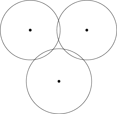
intersection
So in this example the Vietoris-Rips complex is a graph with a 2-simplex, while the Čech complex is just a graph.
One obvious question is: do we still get the benefits of the nerve theorem with Vietoris-Rips complexes? The answer is no, obviously, because the Vietoris-Rips complex and Čech complex in this triangle example have totally different topology! But everything’s not lost. What we can do instead is compare Vietoris-Rips and Čech complexes with related parameters.
Theorem: For all $ \varepsilon > 0$, the following inclusions hold
$$\displaystyle C_{\varepsilon} \subset VR_{\varepsilon} \subset C_{2\varepsilon}$$So if the Čech complexes for both $ \varepsilon$ and $ 2\varepsilon$ are good approximations of the underlying data, then so is the Vietoris-Rips complex. In fact, you can make this chain of inclusions slightly tighter, and if you’re interested you can see Theorem 2.5 in this recent paper of de Silva and Ghrist.
Now your first objection should be that computing a Vietoris-Rips complex still requires exponential time, because you have to scan all subsets for the possibility that they form a simplex. It’s true, but one nice thing about the Vietoris-Rips complex is that it can be represented implicitly as a graph. You just include an edge between two points if their corresponding balls overlap. Once we want to compute the actual simplices in the complex we have to scan for cliques in the graph, so that sucks. But it turns out that computing the graph is the first step in other more efficient methods for computing (or approximating) the VR complex.
Let’s go ahead and write a (trivial) program that computes the graph representation of the Vietoris-Rips complex of a given data set.
import numpy
def naiveVR(points, epsilon):
   points = [numpy.array(x) for x in points]
   vrComplex = [(x,y) for (x,y) in combinations(points, 2) if norm(x - y) < 2*epsilon]
   return numpy.array(vrComplex)
Let’s try running it on a modestly large example: the first frame of the Radiohead music video. It’s got about 12,000 points in $ \mathbb{R}^4$ (x,y,z,intensity), and sadly it takes about twenty minutes. There are a couple of ways to make it more efficient. One is to use specially-crafted data structures for computing threshold queries (i.e., find all points within $ \varepsilon$ of this point). But those are only useful for small thresholds, and we’re interested in sweeping over a range of thresholds. Another is to invoke approximations of the data structure which give rise to “approximate” Vietoris-Rips complexes.
Other stuff
In a future post we’ll implement a method for speeding up the computation of the Vietoris-Rips complex, since this is the primary bottleneck for topological data analysis. But for now the conceptual idea of how Čech complexes and Vietoris-Rips complexes can be used to turn point clouds into simplicial complexes in reasonable ways.
Before we close we should mention that there are other ways to do this. I’ve chosen the algebraic flavor of topological data analysis due to my familiarity with algebra and the work based on this approach. The other approaches have a more geometric flavor, and are based on the Delaunay triangulation, a hallmark of computational geometry algorithms. The two approaches I’ve heard of are called the alpha complex and the flow complex. The downside of these approaches is that, because they are based on the Delaunay triangulation, they have poor scaling in the dimension of the data. Because high dimensional data is crucial, many researchers have been spending their time figuring out how to speed up approximations of the V-R complex. See these slides of Afra Zomorodian for an example.
Until next time!
Want to respond? Send me an email, post a webmention, or find me elsewhere on the internet.