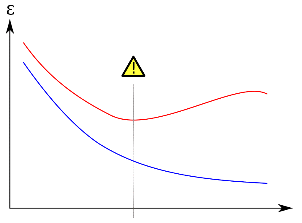
There’s a well-understood phenomenon in machine learning called overfitting. The idea is best shown by a graph:
overfitting
Let me explain. The vertical axis represents the error of a hypothesis. The horizontal axis represents the complexity of the hypothesis. The blue curve represents the error of a machine learning algorithm’s output on its training data, and the red curve represents the generalization of that hypothesis to the real world. The overfitting phenomenon is marker in the middle of the graph, before which the training error and generalization error both go down, but after which the training error continues to fall while the generalization error rises.
The explanation is a sort of numerical version of Occam’s Razor that says more complex hypotheses can model a fixed data set better and better, but at some point a simpler hypothesis better models the underlying phenomenon that generates the data. To optimize a particular learning algorithm, one wants to set parameters of their model to hit the minimum of the red curve.
This is where things get juicy. Boosting, which we covered in gruesome detail previously, has a natural measure of complexity represented by the number of rounds you run the algorithm for. Each round adds one additional “weak learner” weighted vote. So running for a thousand rounds gives a vote of a thousand weak learners. Despite this, boosting doesn’t overfit on many datasets. In fact, and this is a shocking fact, researchers observed that Boosting would hit zero training error, they kept running it for more rounds, and the generalization error kept going down! It seemed like the complexity could grow arbitrarily without penalty.
Schapire, Freund, Bartlett, and Lee proposed a theoretical explanation for this based on the notion of a margin, and the goal of this post is to go through the details of their theorem and proof. Remember that the standard AdaBoost algorithm produces a set of weak hypotheses $ h_i(x)$ and a corresponding weight $ \alpha_i \in [-1,1]$ for each round $ i=1, \dots, T$. The classifier at the end is a weighted majority vote of all the weak learners (roughly: weak learners with high error on “hard” data points get less weight).
Definition: The signed confidence of a labeled example $ (x,y)$ is the weighted sum:
$$\displaystyle \textup{conf}(x) = \sum_{i=1}^T \alpha_i h_i(x)$$The margin of $ (x,y)$ is the quantity $ \textup{margin}(x,y) = y \textup{conf}(x)$. The notation implicitly depends on the outputs of the AdaBoost algorithm via “conf.”
We use the product of the label and the confidence for the observation that $ y \cdot \textup{conf}(x) \leq 0$ if and only if the classifier is incorrect. The theorem we’ll prove in this post is
Theorem: With high probability over a random choice of training data, for any $ 0 < \theta < 1$ generalization error of boosting is bounded from above by
$$\displaystyle \Pr_{\textup{train}}[\textup{margin}(x) \leq \theta] + O \left ( \frac{1}{\theta} (\textup{typical error terms}) \right )$$In words, the generalization error of the boosting hypothesis is bounded by the distribution of margins observed on the training data. To state and prove the theorem more generally we have to return to the details of PAC-learning. Here and in the rest of this post, $ \Pr_D$ denotes $ \Pr_{x \sim D}$, the probability over a random example drawn from the distribution $ D$, and $ \Pr_S$ denotes the probability over a random (training) set of examples drawn from $ D$.
Theorem: Let $ S$ be a set of $ m$ random examples chosen from the distribution $ D$ generating the data. Assume the weak learner corresponds to a finite hypothesis space $ H$ of size $ |H|$, and let $ \delta > 0$. Then with probability at least $ 1 – \delta$ (over the choice of $ S$), every weighted-majority vote function $ f$ satisfies the following generalization bound for every $ \theta > 0$.
$$\displaystyle \Pr_D[y f(x) \leq 0] \leq \Pr_S[y f(x) \leq \theta] + O \left ( \frac{1}{\sqrt{m}} \sqrt{\frac{\log m \log |H|}{\theta^2} + \log(1/\delta)} \right )$$In other words, this phenomenon is a fact about voting schemes, not boosting in particular. From now on, a “majority vote” function $ f(x)$ will mean to take the sign of a sum of the form $ \sum_{i=1}^N a_i h_i(x)$, where $ a_i \geq 0$ and $ \sum_i a_i = 1$. This is the “convex hull” of the set of weak learners $ H$. If $ H$ is infinite (in our proof it will be finite, but we’ll state a generalization afterward), then only finitely many of the $ a_i$ in the sum may be nonzero.
To prove the theorem, we’ll start by defining a class of functions corresponding to “unweighted majority votes with duplicates:”
Definition: Let $ C_N$ be the set of functions $ f(x)$ of the form $ \frac{1}{N} \sum_{i=1}^N h_i(x)$ where $ h_i \in H$ and the $ h_i$ may contain duplicates (some of the $ h_i$ may be equal to some other of the $ h_j$).
Now every majority vote function $ f$ can be written as a weighted sum of $ h_i$ with weights $ a_i$ (I’m using $ a$ instead of $ \alpha$ to distinguish arbitrary weights from those weights arising from Boosting). So any such $ f(x)$ defines a natural distribution over $ H$ where you draw function $ h_i$ with probability $ a_i$. I’ll call this distribution $ A_f$. If we draw from this distribution $ N$ times and take an unweighted sum, we’ll get a function $ g(x) \in C_N$. Call the random process (distribution) generating functions in this way $ Q_f$. In diagram form, the logic goes
$ f \to $ weights $ a_i \to$ distribution over $ H \to$ function in $ C_N$ by drawing $ N$ times according to $ H$.
The main fact about the relationship between $ f$ and $ Q_f$ is that each is completely determined by the other. Obviously $ Q_f$ is determined by $ f$ because we defined it that way, but $ f$ is also completely determined by $ Q_f$ as follows:
$$\displaystyle f(x) = \mathbb{E}_{g \sim Q_f}[g(x)]$$Proving the equality is an exercise for the reader.
Proof of Theorem. First we’ll split the probability $ \Pr_D[y f(x) \leq 0]$ into two pieces, and then bound each piece.
First a probability reminder. If we have two events $ A$ and $ B$ (in what’s below, this will be $ yg(x) \leq \theta/2$ and $ yf(x) \leq 0$, we can split up $ \Pr[A]$ into $ \Pr[A \textup{ and } B] + \Pr[A \textup{ and } \overline{B}]$ (where $ \overline{B}$ is the opposite of $ B$). This is called the law of total probability. Moreover, because $ \Pr[A \textup{ and } B] = \Pr[A | B] \Pr[B]$ and because these quantities are all at most 1, it’s true that $ \Pr[A \textup{ and } B] \leq \Pr[A \mid B]$ (the conditional probability) and that $ \Pr[A \textup{ and } B] \leq \Pr[B]$.
Back to the proof. Notice that for any $ g(x) \in C_N$ and any $ \theta > 0$, we can write $ \Pr_D[y f(x) \leq 0]$ as a sum:
$$\displaystyle \Pr_D[y f(x) \leq 0] =\\\ \Pr_D[yg(x) \leq \theta/2 \textup{ and } y f(x) \leq 0] + \Pr_D[yg(x) > \theta/2 \textup{ and } y f(x) \leq 0]$$Now I’ll loosen the first term by removing the second event (that only makes the whole probability bigger) and loosen the second term by relaxing it to a conditional:
$$\displaystyle \Pr_D[y f(x) \leq 0] \leq \Pr_D[y g(x) \leq \theta / 2] + \Pr_D[yg(x) > \theta/2 \mid yf(x) \leq 0]$$Now because the inequality is true for every $ g(x) \in C_N$, it’s also true if we take an expectation of the RHS over any distribution we choose. We’ll choose the distribution $ Q_f$ to get
$$\displaystyle \Pr_D[yf(x) \leq 0] \leq T_1 + T_2$$And $ T_1$ (term 1) is
$$\displaystyle T_1 = \Pr_{x \sim D, g \sim Q_f} [yg(x) \leq \theta /2] = \mathbb{E}_{g \sim Q_f}[\Pr_D[yg(x) \leq \theta/2]]$$And $ T_2$ is
$$\displaystyle \Pr_{x \sim D, g \sim Q_f}[yg(x) > \theta/2 \mid yf(x) \leq 0] = \mathbb{E}_D[\Pr_{g \sim Q_f}[yg(x) > \theta/2 \mid yf(x) \leq 0]]$$We can rewrite the probabilities using expectations because (1) the variables being drawn in the distributions are independent, and (2) the probability of an event is the expectation of the indicator function of the event.
Now we’ll bound the terms $ T_1, T_2$ separately. We’ll start with $ T_2$.
Fix $ (x,y)$ and look at the quantity inside the expectation of $ T_2$.
$$\displaystyle \Pr_{g \sim Q_f}[yg(x) > \theta/2 \mid yf(x) \leq 0]$$This should intuitively be very small for the following reason. We’re sampling $ g$ according to a distribution whose expectation is $ f$, and we know that $ yf(x) \leq 0$. Of course $ yg(x)$ is unlikely to be large.
Mathematically we can prove this by transforming the thing inside the probability to a form suitable for the Chernoff bound. Saying $ yg(x) > \theta / 2$ is the same as saying $ |yg(x) – \mathbb{E}[yg(x)]| > \theta /2$, i.e. that some random variable which is a sum of independent random variables (the $ h_i$) deviates from its expectation by at least $ \theta/2$. Since the $ y$’s are all $ \pm 1$ and constant inside the expectation, they can be removed from the absolute value to get
$$\displaystyle \leq \Pr_{g \sim Q_f}[g(x) – \mathbb{E}[g(x)] > \theta/2]$$The Chernoff bound allows us to bound this by an exponential in the number of random variables in the sum, i.e. $ N$. It turns out the bound is $ e^{-N \theta^2 / 8}$.
Now recall $ T_1$
$$\displaystyle T_1 = \Pr_{x \sim D, g \sim Q_f} [yg(x) \leq \theta /2] = \mathbb{E}_{g \sim Q_f}[\Pr_D[yg(x) \leq \theta/2]]$$For $ T_1$, we don’t want to bound it absolutely like we did for $ T_2$, because there is nothing stopping the classifier $ f$ from being a bad classifier and having lots of error. Rather, we want to bound it in terms of the probability that $ yf(x) \leq \theta$. We’ll do this in two steps. In step 1, we’ll go from $ \Pr_D$ of the $ g$’s to $ \Pr_S$ of the $ g$’s.
Step 1: For any fixed $ g, \theta$, if we take a sample $ S$ of size $ m$, then consider the event in which the sample probability deviates from the true distribution by some value $ \varepsilon_N$, i.e. the event
$$\displaystyle \Pr_D[yg(x) \leq \theta /2] > \Pr_{S, x \sim S}[yg(x) \leq \theta/2] + \varepsilon_N$$The claim is this happens with probability at most $ e^{-2m\varepsilon_N^2}$. This is again the Chernoff bound in disguise, because the expected value of $ \Pr_S$ is $ \Pr_D$, and the probability over $ S$ is an average of random variables (it’s a slightly different form of the Chernoff bound; see this post for more). From now on we’ll drop the $ x \sim S$ when writing $ \Pr_S$.
The bound above holds true for any fixed $ g,\theta$, but we want a bound over all $ g$ and $ \theta$. To do that we use the union bound. Note that there are only $ (N+1)$ possible choices for a nonnegative $ \theta$ because $ g(x)$ is a sum of $ N$ values each of which is either $ \pm1$. And there are only $ |C_N| \leq |H|^N$ possibilities for $ g(x)$. So the union bound says the above event will occur with probability at most $ (N+1)|H|^N e^{-2m\varepsilon_N^2}$.
If we want the event to occur with probability at most $ \delta_N$, we can judiciously pick
$$\displaystyle \varepsilon_N = \sqrt{(1/2m) \log ((N+1)|H|^N / \delta_N)}$$And since the bound holds in general, we can take expectation with respect to $ Q_f$ and nothing changes. This means that for any $ \delta_N$, our chosen $ \varepsilon_N$ ensures that the following is true with probability at least $ 1-\delta_N$:
$$\displaystyle \Pr_{D, g \sim Q_f}[yg(x) \leq \theta/2] \leq \Pr_{S, g \sim Q_f}[yg(x) \leq \theta/2] + \varepsilon_N$$Now for step 2, we bound the probability that $ yg(x) \leq \theta/2$ on a sample to the probability that $ yf(x) \leq \theta$ on a sample.
Step 2: The first claim is that
$$\displaystyle \Pr_{S, g \sim Q_f}[yg(x) \leq \theta / 2] \leq \Pr_{S} [yf(x) \leq \theta] + \mathbb{E}_{S}[\Pr_{g \sim Q_f}[yg(x) \leq \theta/2 \mid yf(x) \geq \theta]]$$What we did was break up the LHS into two “and”s, when $ yf(x) > \theta$ and $ yf(x) \leq \theta$ (this was still an equality). Then we loosened the first term to $ \Pr_{S}[yf(x) \leq \theta]$ since that is only more likely than both $ yg(x) \leq \theta/2$ and $ yf(x) \leq \theta$. Then we loosened the second term again using the fact that a probability of an “and” is bounded by the conditional probability.
Now we have the probability of $ yg(x) \leq \theta / 2$ bounded by the probability that $ yf(x) \leq 0$ plus some stuff. We just need to bound the “plus some stuff” absolutely and then we’ll be done. The argument is the same as our previous use of the Chernoff bound: we assume $ yf(x) \geq \theta$, and yet $ yg(x) \leq \theta / 2$. So the deviation of $ yg(x)$ from its expectation is large, and the probability that happens is exponentially small in the amount of deviation. The bound you get is
$$\displaystyle \Pr_{g \sim Q}[yg(x) \leq \theta/2 \mid yf(x) > \theta] \leq e^{-N\theta^2 / 8}.$$And again we use the union bound to ensure the failure of this bound for any $ N$ will be very small. Specifically, if we want the total failure probability to be at most $ \delta$, then we need to pick some $ \delta_j$’s so that $ \delta = \sum_{j=0}^{\infty} \delta_j$. Choosing $ \delta_N = \frac{\delta}{N(N+1)}$ works.
Putting everything together, we get that with probability at least $ 1-\delta$ for every $ \theta$ and every $ N$, this bound on the failure probability of $ f(x)$:
$$\displaystyle \Pr_{x \sim D}[yf(x) \leq 0] \leq \Pr_{S, x \sim S}[yf(x) \leq \theta] + 2e^{-N \theta^2 / 8} + \sqrt{\frac{1}{2m} \log \left ( \frac{N(N+1)^2 |H|^N}{\delta} \right )}.$$This claim is true for every $ N$, so we can pick $ N$ that minimizes it. Doing a little bit of behind-the-scenes calculus that is left as an exercise to the reader, a tight choice of $ N$ is $ (4/ \theta)^2 \log(m/ \log |H|)$. And this gives the statement of the theorem.
$$\square$$We proved this for finite hypothesis classes, and if you know what VC-dimension is, you’ll know that it’s a central tool for reasoning about the complexity of infinite hypothesis classes. An analogous theorem can be proved in terms of the VC dimension. In that case, calling $ d$ the VC-dimension of the weak learner’s output hypothesis class, the bound is
$$\displaystyle \Pr_D[yf(x) \leq 0] \leq \Pr_S[yf(x) \leq \theta] + O \left ( \frac{1}{\sqrt{m}} \sqrt{\frac{d \log^2(m/d)}{\theta^2} + \log(1/\delta)} \right )$$How can we interpret these bounds with so many parameters floating around? That’s where asymptotic notation comes in handy. If we fix $ \theta \leq 1/2$ and $ \delta = 0.01$, then the big-O part of the theorem simplifies to $ \sqrt{(\log |H| \cdot \log m) / m}$, which is easier to think about since $ (\log m)/m$ goes to zero very fast.
Now the theorem we just proved was about any weighted majority function. The question still remains: why is AdaBoost good? That follows from another theorem, which we’ll state and leave as an exercise (it essentially follows by unwrapping the definition of the AdaBoost algorithm from last time).
Theorem: Suppose that during AdaBoost the weak learners produce hypotheses with training errors $ \varepsilon_1, \dots , \varepsilon_T$. Then for any $ \theta$,
$$\displaystyle \Pr_{(x,y) \sim S} [yf(x) \leq \theta] \leq 2^T \prod_{t=1}^T \sqrt{\varepsilon_t^{(1-\theta)} (1-\varepsilon_t)^{(1+\theta)}}$$Let’s interpret this for some concrete numbers. Say that $ \theta = 0$ and $ \varepsilon_t$ is any fixed value less than $ 1/2$. In this case the term inside product becomes $ \sqrt{\varepsilon (1-\varepsilon)} < 1/2$ and the whole bound tends exponentially quickly to zero in the number of rounds $ T$. On the other hand, if we raise $ \theta$ to about 1/3, then in order to maintain the LHS tending to zero we would need $ \varepsilon < \frac{1}{4} ( 3 – \sqrt{5} )$ which is about 20% error.
If you’re interested in learning more about Boosting, there is an excellent book by Freund and Schapire (the inventors of boosting) called Boosting: Foundations and Algorithms. There they include a tighter analysis based on the idea of Rademacher complexity. The bound I presented in this post is nice because the proof doesn’t require any machinery past basic probability, but if you want to reach the cutting edge of knowledge about boosting you need to invest in the technical stuff.
Until next time!
Want to respond? Send me an email, post a webmention, or find me elsewhere on the internet.