Update 2017-01-09: Laci claims to have found a workaround to the previously posted error, and the claim is again quasipolynoimal time! Updated arXiv paper to follow.
Update 2017-01-04: Laci has posted an update on his paper. The short version is that one small step of his analysis was not quite correct, and the result is that his algorithm is sub-exponential, but not quasipolynomial time. The fact that this took over a year to sort out is a testament to the difficulty of the mathematics and the skill of the mathematicians involved. Even the revised result is still a huge step forward in the analysis of graph isomorphism. Finally, this should reinforce how we should think about progress in mathematics: it comes in fits and starts, with occasional steps backward.
Update 2015-12-13: Laci has posted a preprint on arXiv. It’s quite terse, but anyone who is comfortable with the details sketched in this article should have a fine time (albeit a long time) reading it.
Update 2015-11-21: Ken Regan and Dick Lipton posted an article with some more details, and a high level overview of how the techniques fit into the larger picture of CS theory.
Update 2015-11-16: Laci has posted the talk on his website. It’s an hour and a half long, and I encourage you to watch it if you have the time 🙂
Laszlo Babai has claimed an astounding theorem, that the Graph Isomorphism problem can be solved in quasipolynomial time (now outdated; see Update 2017-01-04 above). On Tuesday I was at Babai’s talk on this topic (he has yet to release a preprint), and I’ve compiled my notes here. As in Babai’s talk, familiarity with basic group theory and graph theory is assumed, and if you’re a casual (i.e., math-phobic) reader looking to understand what the fuss is all about, this is probably not the right post for you. This post is research level theoretical computer science. We’re here for the juicy, glorious details.
Note: this blog post will receive periodic updates as my understanding of the details improve.
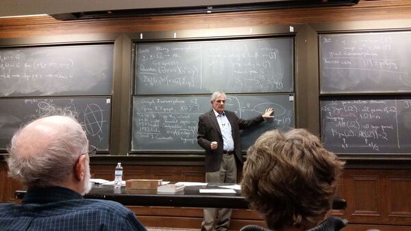
Laci during his lecture.
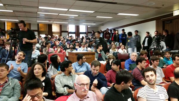
Standing room only at Laci's talk.
Background on Graph Isomorphism
I’ll start by giving a bit of background into why Graph Isomorphism (hereafter, GI) is such a famous problem, and why this result is important. If you’re familiar with graph isomorphism and the basics of complexity theory, skip to the next section where I get into the details.
GI is the following problem: given two graphs $ G = (V_G, E_G), H = (V_H, E_H)$, determine whether the graphs are isomorphic, that is, whether there is a bijection $ f : V_G \to V_H$ such that $ u,v$ are connected in $ G$ if and only if $ f(u), f(v)$ are connected in $ H$. Informally, GI asks whether it’s easy to tell from two drawings of a graph whether the drawings actually represent the same graph. If you’re wondering why this problem might be hard, check out the following picture of the same graph drawn in three different ways.
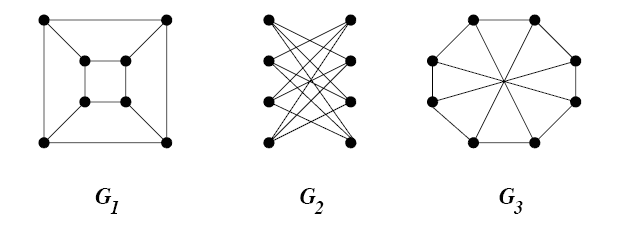
GI-example
Indeed, a priori the worst-case scenario is that one would have to try all $ n!$ ways to rearrange the nodes of the first graph and see if one rearrangement achieves the second graph. The best case scenario is that one can solve this problem efficiently, that is, with an algorithm whose worst-case runtime on graphs with $ n$ nodes and $ m$ edges is polynomial in $ n$ and $ m$ (this would show that GI is in the class P). However, nobody knows whether there is a polynomial time algorithm for GI, and it’s been a big open question in CS theory for over forty years. This is the direction that Babai is making progress toward, showing that there are efficient algorithms. He didn’t get a polynomial time algorithm, but he got something quite close, which is why everyone is atwitter.
It turns out that telling whether two graphs are isomorphic has practical value in some applications. I hear rumor that chemists use it to search through databases of chemicals for one with certain properties (one way to think of a chemical compound is as a graph). I also hear that some people use graph isomorphism to compare files, do optical character recognition, and analyze social networks, but it seems highly probable to me that GI is not the central workhorse (or even a main workhorse) in these fields. Nevertheless, the common understanding is that pretty much anybody who needs to solve GI on a practical level can do so efficiently. The heuristics work well. Even in Babai’s own words, getting better worst-case algorithms for GI is purely a theoretical enterprise.
So if GI isn’t vastly important for real life problems, why are TCS researchers so excited about it?
Well it’s known that GI is in the class NP, meaning if two graphs are isomorphic you can give me a short proof that I can verify in polynomial time (the proof is just a description of the function $ f : V_G \to V_H$). And if you’ll recall that inside NP there is this class called NP-complete, which are the “hardest” problems in NP. Now most problems in NP that we care about are also NP-complete, but it turns out GI is not known to be NP-complete either. Now, for all we know P = NP and then the question about GI is moot, but in the scenario that most people believe P and NP are different, so it leaves open the question of where GI lies: does it have efficient algorithms or not?
So we have a problem which is in NP, it’s not known to be in P, and it’s not known to be NP-complete. One obvious objection is that it might be neither. In fact, there’s a famous theorem of Ladner that says if P is different from NP, then there must be problems in NP, not in P, and not NP-complete. Such problems are called “NP-intermediate.” It’s perfectly reasonable that GI is one of these problems. But there’s a bit of a catch.
See, Ladner’s theorem doesn’t provide a natural problem which is NP intermediate; what Ladner did in his theorem was assume P is not NP, and then use that assumption to invent a new problem that he could prove is NP intermediate. If you come up with a problem whose only purpose is to prove a theorem, then the problem is deemed unnatural. In fact, there is no known “natural” NP-intermediate problem (assuming P is not NP). The pattern in CS theory is actually that if we find a problem that might be NP-intermediate, someone later finds an efficient algorithm for it or proves it’s NP-complete. There is a small and dwindling list of such problems. I say dwindling because not so long ago the problem of telling whether an integer is prime was in this list. The symptoms are that one first solves the problem on many large classes of special cases (this is true of GI) or one gets a nice quasipolynomial-time algorithm (Babai’s claimed new result), and then finally it falls into P. In fact, there is even stronger evidence against it being NP-complete: if GI were NP-complete, the polynomial hierarchy would collapse. To the layperson, the polynomial hierarchy is abstruse complexity theoretic technical hoo-hah, but suffice it to say that most experts believe the hierarchy does not collapse, so this counts as evidence.
So indeed, it could be that GI will become the first ever problem which is NP-intermediate (assuming P is not NP), but from historical patterns it seems more likely that it will fall into P. So people are excited because it’s tantalizing: everyone believes it should be in P, but nobody can prove it. It’s right at the edge of the current state of knowledge about the theoretical capabilities and limits of computation.
This is the point at which I will start assuming some level of mathematical maturity.
The Main Result
The specific claim about graph isomorphism being made is the following:
Theorem: There is a deterministic algorithm for GI which runs in time $ 2^{O(\log^c(n))}$ for some constant $ c$.
This is an improvement over the best previously known algorithm which had runtime $ 2^{\sqrt{n \log n}}$. Note the $ \sqrt{n}$ in the exponent has been eliminated, which is a huge difference. Quantities which are exponential in some power of a logarithm are called “quasipolynomial.”
But the main result is actually a quasipolynomial time algorithm for a different, more general problem called string automorphism. In this context, given a set $ X$ a string is a function from $ X$ to some finite alphabet (really it is a coloring of $ X$, but we are going to use colorings in the usual sense later so we have to use a new name here). If the set $ X$ is given a linear ordering then strings on $ X$ really correspond to strings of length $ |X|$ over the alphabet. We will call strings $ x,y \in X$.
Now given a set $ X$ and a group $ G$ acting on $ X$, there is a natural action of $ G$ on strings over $ X$, denoted $ x^\sigma$, by permuting the indices $ x^{\sigma}(i) = x(\sigma(i))$. So you can ask the natural question: given two strings $ x,y$ and a representation of a group $ G$ acting on $ X$ by a set of generating permutations of $ G$, is there a $ \sigma \in G$ with $ x^\sigma = y$? This problem is called the string isomorphism problem, and it’s clearly in NP.
Now if you call $ \textup{ISO}_G(x,y)$ the set of all permutations in $ G$ that map $ x$ to $ y$, and you call $ \textup{Aut}_G(x) = \textup{ISO}_G(x,x)$, then the actual theorem Babai claims to have proved is the following.
Theorem: Given a generating set for a group $ G$ of permutations of a set $ X$ and a string $ x$, there is a quasipolynomial time algorithm which produces a generating set of the subgroup $ \textup{Aut}_G(x)$ of $ G$, i.e. the string automorphisms of $ x$ that lie in in $ G$.
It is not completely obvious that GI reduces to the automorphism problem, but I will prove it does in the next section. Furthermore, the overview of Babai’s proof of the theorem follows an outline laid out by Eugene Luks in 1982, which involves a divide-and-conquer method for splitting the analysis of $ \textup{Aut}_G(x)$ into simpler and simpler subgroups as they are found.
Luks’s program
Eugene Luks was the first person to incorporate “serious group theory” (Babai’s words) into the study of graph isomorphism. Why would group theory help in a question about graphs? Let me explain with a lemma.
Lemma: GI is polynomial-time reducible to the problem of computing, given a graph $ X$, a list of generators for the automorphism group of $ G$, denoted $ \textup{Aut}(X)$.
Proof. Without loss of generality suppose $ X_1, X_2$ are connected graphs. If we want to decide whether $ X_1, X_2$ are isomorphic, we may form the disjoint union $ X = X_1 \cup X_2$. It is easy to see that $ X_1$ and $ X_2$ are isomorphic if and only if some $ \sigma \in \textup{Aut}(X)$ swaps $ X_1$ and $ X_2$. Indeed, if any automorphism with this property exists, every generating set of $ \textup{Aut}(G)$ must contain one.
$$\square$$Similarly, the string isomorphism problem reduces to the problem of computing a generating set for $ \textup{Aut}_G(x)$ using a similar reduction to the one above. As a side note, while $ \textup{ISO}_G(x,y)$ can be exponentially large as a set, it is either the empty set, or a coset of $ \textup{Aut}_G(x)$ by any element of $ \textup{ISO}_G(x,y)$. So there are group-theoretic connections between the automorphism group of a string and the isomorphisms between two strings.
But more importantly, computing the automorphism group of a graph reduces to computing the automorphism subgroup of a particular group for a given string in the following way. Given a graph $ X$ on a vertex set $ V = \{ 1, 2, \dots, v \}$ write $ X$ as a binary string on the set of unordered pairs $ Z = \binom{V}{2}$ by mapping $ (i,j) \to 1$ if and only if $ i$ and $ j$ are connected by an edge. The alphabet size is 2. Then $ \textup{Aut}(X)$ (automorphisms of the graph) induces an action on strings as a subgroup $ G_X$ of $ \textup{Aut}(Z)$ (automorphisms of strings). These induced automorphisms are exactly those which preserve proper encodings of a graph. Moreover, any string automorphism in $ G_X$ is an automorphism of $ X$ and vice versa. Note that since $ Z$ is larger than $ V$ by a factor of $ v^2$, the subgroup $ G_X$ is much smaller than all of $ \textup{Aut}(Z)$.
Moreover, $ \textup{Aut}(X)$ sits inside the full symmetry group $ \textup{Sym}(V)$ of $ V$, the vertex set of the starting graph, and $ \textup{Sym}(V)$ also induces an action $ G_V$ on $ Z$. The inclusion is
$$\displaystyle \textup{Aut}(X) \subset \textup{Sym}(V)$$induces
$$\displaystyle G_X = \textup{Aut}(\textup{Enc}(X)) \subset G_V \subset \textup{Aut}(Z)$$I.e.,
Call $ G = G_V$ the induced subgroup of permutations of strings-as-graphs. Now we just have some subgroup of permutations $ G$ of $ \textup{Aut}(Z)$, and we want to find a generating set for $ \textup{Aut}_G(x)$ (where $ x$ happens to be the encoding of a graph). That is exactly the string automorphism problem. Reduction complete.
Now the basic idea to compute $ \textup{Aut}_G(x)$ is to start from the assumption that $ \textup{Aut}_G(x) = G$. We know it’s a subgroup, so it could be all of $ G$; in terms of GI if this assumption were true it would mean the starting graph was the complete graph, but for string automorphism in general $ G$ can be whatever. Then we try to refute this belief by finding additional structure in $ \textup{Aut}_G(x)$, either by breaking it up into smaller pieces (say, orbits) or by constructing automorphisms in it. That additional structure allows us to break up $ G$ in a way that $ \textup{Aut}_G(x)$ is a subgroup of the product of the corresponding factors of $ G$.
The analogy that Babai used, which goes back to graphs, is the following. If you have a graph $ X$ and you want to know its automorphisms, one thing you can do is to partition the vertices by degree. You know that an automorphism has to preserve the degree of an individual vertex, so in particular you can break up the assumption that $ \textup{Aut}(X) = \textup{Sym}(V)$ into the fact that $ \textup{Aut}(X)$ must be a subgroup of the product of the symmetry groups of the pieces of the partition; then you recurse. In this way you’ve hugely reduced the total number of automorphisms you need to consider. When the degrees get small enough you can brute-force search for automorphisms (and there is some brute-force searching in putting the pieces back together). But of course this approach fails miserably in the first step you start with a regular graph, so one would need to look for other kinds of structure.
One example is an equitable partition, which is a partition of vertices by degree relative to vertices in other blocks of the partition. So a vertex which has degree 3 but two degree 2 neighbors would be in a different block than a vertex with degree 3 and only 1 neighbor of degree 2. Finding these equitable partitions (which can be done in polynomial time) is one of the central tools used to attack GI. As an example of why it can be very helpful: in many regimes a Erdos-Renyi random graph has asymptotically almost surely a coarsest equitable partition which consists entirely of singletons. This is despite the fact that the degree sequences themselves are tightly constrained with high probability. This means that, if you’re given two Erdos-Renyi random graphs and you want to know whether they’re isomorphic, you can just separately compute the coarsest equitable partition for each one and see if the singleton blocks match up. That is your isomorphism.
Even still, there are many worst case graphs that resist being broken up by an equitable partition. A hard example is known as the Johnson graph, which we’ll return to later.
For strings the sorts of structures to look for are even more refined than equitable partitions of graphs, because the automorphism group of a graph can be partitioned into orbits which preserve the block structure of an equitable partition. But it still turns out that Johnson graphs admit parts of the automorphism group that can’t be broken up much by orbits.
The point is that when some useful substructure is found, it will “make progress” toward the result by breaking the problem into many pieces (say, $ n^{\log n}$ pieces) where each piece has size $ 9/10$ the size of the original. So you get a recursion in the amount of time needed which looks like $ f(n) \leq n^{\log n} f(9n/10)$. If you call $ q(n) = n^{\log n}$ the quasipolynomial factor, then solving the recurrence gives $ f(n) \leq q(n)^{O(\log n)}$ which only adds an extra log factor in the exponent. So you keep making progress until the problem size is polylogarithmic, and then you brute force it and put the pieces back together in quasipolynomial time.
Two main lemmas, which are theorems in their own right
This is where the details start to get difficult, in part because Babai jumped back and forth between thinking of the object as a graph and as a string. The point of this in the lecture was to illustrate both where the existing techniques for solving GI (which were in terms of finding canonical graph substructures in graphs) break down.
The central graph-theoretic picture is that of “individualizing” a vertex by breaking it off from an existing equitable partition, which then breaks the equitable partition structure so you need to do some more (polytime) work to further refine it into an equitable partition again. But the point is that you can take all the vertices in a block, pick all possible ways to individualize them by breaking them into smaller blocks. If you traverse these possibilities in a canonical order, you will eventually get down to a partition of singletons, which is your “canonical labeling” of the graph. And if you do this process with two different graphs and you get to different canonical labelings, you had to have started with non-isomorphic graphs.
The problem is that when you get to a coarsest equitable partition, you may end up with blocks of size $ \sqrt{n}$, meaning you have an exponential number of individualizations to check. This is the case with Johnson graphs, and in fact if you have a Johnson graph $ J(m,t)$ which has $ \binom{m}{t}$ vertices and you individualize fewer than $ m/10t$ if them, then you will only get down to blocks of size polynomially smaller than $ \binom{m}{t}$, which is too big if you want to brute force check all individualizations of a block.
The main combinatorial lemma that Babai proves to avoid this problem is that the Johnson graphs are the only obstacle to finding efficient partitions.
Theorem (Babai 15): If $ X$ is a regular graph on $ m$ vertices, then by individualizing a polylog number of vertices we can find one of the three following things:
- A canonical coloring with each color class having at most 90% of all the nodes.
- A canonical equipartition of some subset of the vertices that has at least 90% of the nodes (i.e. a big color class from (1)).
- A canonically embedded Johnson graph on at least 90% of the nodes.
[Edit: I think that what Babai means by a “canonical coloring” is an equitable partition of the nodes (not to be confused with an equipartition), but I am not entirely sure. I have changed the language to reflect more clearly what was in the talk as opposed to what I think I understood from doing additional reading.]
The first two are apparently the “easy” cases in the sense that they allow for simple recursion that has already been known before Babai’s work. The hard part is establishing the last case (and this is the theorem whose proof sketch he has deferred for two more weeks). But once you have such a Johnson graph your life is much better, because (for a reason I did not understand) you can recurse on a problem of size roughly the square root of the starting size.
In discussing Johnson graphs, Babai said they were a source of “unspeakable misery” for people who want to solve GI quickly. At the same time, it is a “curse and a blessing,” as once you’ve found a Johnson graph embedded in your problem you can recurse to much smaller instances. This routine to find one of these three things is called the “split-or-Johnson” routine.
The analogue for strings (I believe this is true, but I’m a bit fuzzy on this part) is to find a “canonical” $ k$-ary relational structure (where $ k$ is polylog in size) with some additional condition on the size of alternating subgroups of the automorphism group of the $ k$-ary relational structure. Then you can “individualize” the points in the base of this relational structure and find analogous partitions and embedded Johnson schemes (a special kind of combinatorial design).
One important fact to note is that the split-or-Johnson routine breaks down at $ \log^3(n)$ size, and Babai has counterexamples that say his result is tight, so getting GI in P would have to bypass this barrier with a different idea.
The second crucial lemma has to do with giant homomorphisms, and this is the method by which Babai constructs automorphisms that bound $ \textup{Aut}_G(x)$ from below. As opposed to the split-or-Johnson lemma, which finds structure to bound the group from above by breaking it into simpler pieces. Fair warning: one thing I don’t yet understand is how these two routines interact in the final algorithm. My guess is they are essentially run in parallel (or alternate), but that guess is as good as wild.
Definition: A homomorphism $ \varphi: G \to S_m$ is called giant if the image of $ G$ is either the alternating group $ A_n$ or else all of $ S_m$. I.e. $ \varphi$ is surjective, or almost so. Let $ \textup{Stab}_G(x)$ denote the stabilizer subgroup of $ x \in G$. Then $ x$ is called “affected” by $ \varphi$ if $ \varphi|_{\textup{Stab}_g(x)}$ is not giant.
The central tool in Babai’s algorithm is the dichotomy between points that are affected and those that are not. The ability to decide this property in quasipolynomial time is what makes the divide and conquer work.
There is one deep theorem he uses that relates affected points to giant homomorphisms:
Theorem (Unaffected Stabilizer Theorem): Let $ \varphi: G \to S_m$ be a giant homomorphism and $ U \subset G$ the set of unaffected elements. Let $ G_{(U)}$ be the pointwise stabilizer of $ U$, and suppose that $ m > \textup{max}(8, 2 + \log_2 n)$. Then the restriction $ \varphi : G_{(U)} \to S_m$ is still giant.
Babai claimed this was a nontrivial theorem, not because the proof is particularly difficult, but because it depends on the classification of finite simple groups. He claimed it was a relatively straightforward corollary, but it appears that this does not factor into the actual GI algorithm constructively, but only as an assumption that a certain loop invariant will hold.
To recall, we started with this assumption that $ \textup{Aut}_G(x)$ was the entire symmetry group we started with, which is in particular an assumption that the inclusion $ \varphi \to S_m$ is giant. Now you want to refute this hypothesis, but you can’t look at all of $ S_m$ because even the underlying set $ m$ has too many subsets to check. But what you can do is pick a test set $ A \subset [m]$ where $ |A|$ is polylogarithmic in size, and test whether the restriction of $ \varphi$ to the test set is giant in $ \textup{Sym}(A)$. If it is giant, we call $ A$ full.
Theorem (Babai 15): One can test the property of a polylogarithmic size test set being full in quasipolynomial time in m.
Babai claimed it should be surprising that fullness is a quasipolynomial time testable property, but more surprising is that regardless of whether it’s full or not, we can construct an explicit certificate of fullness or non-fullness. In the latter case, one can come up with an explicit subgroup which contains the image of the projection of the automorphism group onto the symmetry group of the test set. In addition, given two test sets $ A,B$, one can efficiently compare the action between the two different test sets. And finding these non-full test sets is what allows one to construct the $ k$-ary relations. So the output of this lower bound technique informs the upper bound technique of how to proceed.
The other outcome is that $ A$ could be full, and coming up with a certificate of fullness is harder. The algorithm sketched below claims to do it, and it involves finding enough “independent” automorphisms to certify that the projection is giant.
Now once you try all possible test sets, which gives $ \binom{m}{k}^2$ many certificates (a quasipolynomial number), one has to aggregate them into a full automorphism of $ x$, which Babai assured us was a group theoretic exercise.
The algorithm to test fullness (and construct a certificate) he called the Local Certificates Algorithm. It was sketched as follows: you are given as input a set $ A$ and a group $ G_A \subset G$ being the setwise stabilizer of $ A$ under $ \psi_A : G_A \to \textup{Sym}(A)$. Now let $ W$ be the group elements affected by $ \psi_A$. You can be sure that at least one point is affected. Now you stabilize on $ W$ and get a refined subgroup of $ G_A$, which you can use to compute newly affected elements, growing $ W$ in each step. By the unaffected stabilizer theorem, this preserves gianthood. Furthermore, in each step you get layers of $ W$, and all of the stabilizers respect the structure of the previous layers. Babai described this as adding on “layers of a beard.”
The termination of this is either when $ W$ stops growing, in which case the projection is giant and $ W$ is our certificate of fullness (i.e. we get a rich family of automorphisms that are actually in our target automorphism group), or else we discover the projected ceases to be giant and $ W$ is our certificate of non-fullness. Indeed, the subgroup generated by these layers is a subgroup of $ \textup{Aut}_G(x)$, and the subgroup generated by the elements of a non-fullness certificate contain the automorphism group.
Not enough details?
This was supposed to be just a high-level sketch of the algorithm, and Babai is giving two more talks elaborating on the details. Unfortunately, I won’t be able to make it to his second talk in which he’ll discuss some of the core group theoretic ideas that go into the algorithm. I will, however, make it to his third talk in which he will sketch the proof of the split-or-Johnson routine. That is in two weeks from the time of this writing, and I will update this post with any additional insights then.
Babai has not yet released a preprint, and when I asked him he said “soon, soon.” Until then 🙂
This blog post is based on my personal notes from Laszlo Babai’s lecture at the University of Chicago on November 10, 2015. At the time of this writing, Babai’s work has not been peer reviewed, and my understanding of his lectures has large gaps and may be faulty. Do not put your life in danger based on information in this post.
Want to respond? Send me an email, post a webmention, or find me elsewhere on the internet.