Here’s a bit of folklore I often hear (and retell) that’s somewhere between a joke and deep wisdom: if you’re doing a software interview that involves some algorithms problem that seems hard, your best bet is to use hash tables.
More succinctly put: Google loves hash tables.
As someone with a passion for math and theoretical CS, it’s kind of silly and reductionist. But if you actually work with terabytes of data that can’t fit on a single machine, it also makes sense.
But to understand why hash tables are so applicable, you should have at least a fuzzy understanding of the math that goes into it, which is surprisingly unrelated to the actual act of hashing. Instead it’s the guarantees that a “random enough” hash provides that makes it so useful. The basic intuition is that if you have an algorithm that works well assuming the input data is completely random, then you can probably get a good guarantee by preprocessing the input by hashing.
In this post I’ll explain the details, and show the application to an important problem that one often faces in dealing with huge amounts of data: how to allocate resources efficiently (load balancing). As usual, all of the code used in the making of this post is available on Github.
Next week, I’ll follow this post up with another application of hashing to estimating the number of distinct items in a set that’s too large to store in memory.
Families of Hash Functions
To emphasize which specific properties of hash functions are important for a given application, we start by introducing an abstraction: a hash function is just some computable function that accepts strings as input and produces numbers between 1 and $ n$ as output. We call the set of allowed inputs $ U$ (for “Universe”). A family of hash functions is just a set of possible hash functions to choose from. We’ll use a scripty $ \mathscr{H}$ for our family, and so every hash function $ h$ in $ \mathscr{H}$ is a function $ h : U \to \{ 1, \dots, n \}$.
You can use a single hash function $ h$ to maintain an unordered set of objects in a computer. The reason this is a problem that needs solving is because if you were to store items sequentially in a list, and if you want to determine if a specific item is already in the list, you need to potentially check every item in the list (or do something fancier). In any event, without hashing you have to spend some non-negligible amount of time searching. With hashing, you can choose the location of an element $ x \in U$ based on the value of its hash $ h(x)$. If you pick your hash function well, then you’ll have very few collisions and can deal with them efficiently. The relevant section on Wikipedia has more about the various techniques to deal with collisions in hash tables specifically, but we want to move beyond that in this post.
Here we have a family of random hash functions. So what’s the use of having many hash functions? You can pick a hash randomly from a “good” family of hash functions. While this doesn’t seem so magical, it has the informal property that it makes arbitrary data “random enough,” so that an algorithm which you designed to work with truly random data will also work with the hashes of arbitrary data. Moreover, even if an adversary knows $ \mathscr{H}$ and knows that you’re picking a hash function at random, there’s no way for the adversary to manufacture problems by feeding bad data. With overwhelming probability the worst-case scenario will not occur. Our first example of this is in load-balancing.
Load balancing and 2-uniformity
You can imagine load balancing in two ways, concretely and mathematically. In the concrete version you have a public-facing server that accepts requests from users, and forwards them to a back-end server which processes them and sends a response to the user. When you have a billion users and a million servers, you want to forward the requests in such a way that no server gets too many requests, or else the users will experience delays. Moreover, you’re worried that the League of Tanzanian Hackers is trying to take down your website by sending you requests in a carefully chosen order so as to screw up your load balancing algorithm.
The mathematical version of this problem usually goes with the metaphor of balls and bins. You have some collection of $ m$ balls and $ n$ bins in which to put the balls, and you want to put the balls into the bins. But there’s a twist: an adversary is throwing balls at you, and you have to put them into the bins before the next ball comes, so you don’t have time to remember (or count) how many balls are in each bin already. You only have time to do a small bit of mental arithmetic, sending ball $ i$ to bin $ f(i)$ where $ f$ is some simple function. Moreover, whatever rule you pick for distributing the balls in the bins, the adversary knows it and will throw balls at you in the worst order possible.

A young man applying his knowledge of balls and bins. That’s totally what he’s doing.
There is one obvious approach: why not just pick a uniformly random bin for each ball? The problem here is that we need the choice to be persistent. That is, if the adversary throws the same ball at us a second time, we need to put it in the same bin as the first time, and it doesn’t count toward the overall load. This is where the ball/bin metaphor breaks down. In the request/server picture, there is data specific to each user stored on the back-end server between requests (a session), and you need to make sure that data is not lost for some reasonable period of time. And if we were to save a uniform random choice after each request, we’d need to store a number for every request, which is too much. In short, we need the mapping to be persistent, but we also want it to be “like random” in effect.
So what do you do? The idea is to take a “good” family of hash functions $ \mathscr{H}$, pick one $ h \in \mathscr{H}$ uniformly at random for the whole game, and when you get a request/ball $ x \in U$ send it to server/bin $ h(x)$. Note that in this case, the adversary knows your universal family $ \mathscr{H}$ ahead of time, and it knows your algorithm of committing to some single randomly chosen $ h \in \mathscr{H}$, but the adversary does not know which particular $ h$ you chose.
The property of a family of hash functions that makes this strategy work is called 2-universality.
Definition: A family of functions $ \mathscr{H}$ from some universe $ U \to \{ 1, \dots, n \}$. is called 2-universal if, for every two distinct $ x, y \in U$, the probability over the random choice of a hash function $ h$ from $ \mathscr{H}$ that $ h(x) = h(y)$ is at most $ 1/n$. In notation,
$$\displaystyle \Pr_{h \in \mathscr{H}}[h(x) = h(y)] \leq \frac{1}{n}$$I’ll give an example of such a family shortly, but let’s apply this to our load balancing problem. Our load-balancing algorithm would fail if, with even some modest probability, there is some server that receives many more than its fair share ($ m/n$) of the $ m$ requests. If $ \mathscr{H}$ is 2-universal, then we can compute an upper bound on the expected load of a given server, say server 1. Specifically, pick any element $ x$ which hashes to 1 under our randomly chosen $ h$. Then we can compute an upper bound on the expected number of other elements that hash to 1. In this computation we’ll only use the fact that expectation splits over sums, and the definition of 2-universal. Call $ \mathbf{1}_{h(y) = 1}$ the random variable which is zero when $ h(y) \neq 1$ and one when $ h(y) = 1$, and call $ X = \sum_{y \in U} \mathbf{1}_{h(y) = 1}$. In words, $ X$ simply represents the number of inputs that hash to 1. Then
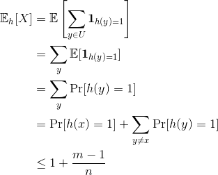
So in expectation we can expect server 1 gets its fair share of requests. And clearly this doesn’t depend on the output hash being 1; it works for any server. There are two obvious questions.
- How do we measure the risk that, despite the expectation we computed above, some server is overloaded?
- If it seems like (1) is on track to happen, what can you do?
For 1 we’re asking to compute, for a given deviation $ t$, the probability that $ X – \mathbb{E}[X] > t$. This makes more sense if we jump to multiplicative factors, since it’s usually okay for a server to bear twice or three times its usual load, but not like $ \sqrt{n}$ times more than it’s usual load. (Industry experts, please correct me if I’m wrong! I’m far from an expert on the practical details of load balancing.)
So we want to know what is the probability that $ X – \mathbb{E}[X] > t \cdot \mathbb{E}[X]$ for some small number $ t$, and we want this to get small quickly as $ t$ grows. This is where the Chebyshev inequality becomes useful. For those who don’t want to click the link, for our sitauation Chebyshev’s inequality is the statement that, for any random variable $ X$
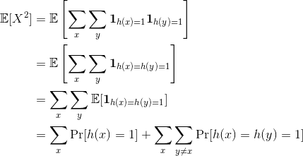
$$\displaystyle \Pr[|X – \mathbb{E}[X]| > t\mathbb{E}[X]] \leq \frac{\textup{Var}[X]}{t^2 \mathbb{E}^2[X]}.$$So all we need to do is compute the variance of the load of a server. It’s a bit of a hairy calculation to write down, but rest assured it doesn’t use anything fancier than the linearity of expectation and 2-universality. Let’s dive in. We start by writing the definition of variance as an expectation, and then we split $ X$ up into its parts, expand the product and group the parts.
$$\displaystyle \textup{Var}[X] = \mathbb{E}[(X – \mathbb{E}[X])^2] = \mathbb{E}[X^2] – (\mathbb{E}[X])^2$$The easy part is $ (\mathbb{E}[X])^2$, it’s just $ (1 + (m-1)/n)^2$, and the hard part is $ \mathbb{E}[X^2]$. So let’s compute that
In order to continue (and get a reasonable bound) we need an additional property of our hash family which is not immediately spelled out by 2-universality. Specifically, we need that for every $ h$ and $ i$, $ \Pr_x[h(x) = i] = O(\frac{1}{n})$. In other words, each hash function should evenly split the inputs across servers.
The reason this helps is because we can split $ \Pr[h(x) = h(y) = 1]$ into $ \Pr[h(x) = h(y) \mid h(x) = 1] \cdot \Pr[h(x) = 1]$. Using 2-universality to bound the left term, this quantity is at most $ 1/n^2$, and since there are $ \binom{m}{2}$ total terms in the double sum above, the whole thing is at most $ O(m/n + m^2 / n^2) = O(m^2 / n^2)$. Note that in our big-O analysis we’re assuming $ m$ is much bigger than $ n$.
Sweeping some of the details inside the big-O, this means that our variance is $ O(m^2/n^2)$, and so our bound on the deviation of $ X$ from its expectation by a multiplicative factor of $ t$ is at most $ O(1/t^2)$.
Now we computed a bound on the probability that a single server is not overloaded, but if we want to extend that to the worst-case server, the typical probability technique is to take the union bound over all servers. This means we just add up all the individual bounds and ignore how they relate. So the probability that some server has a load more than a multiplicative factor of $ t$ is bounded from above $ O(n/t^2)$. This is only less than one when $ t = \Omega(\sqrt{n})$, so all we can say with this analysis is that (with some small constant probability) no server will have a load worse than $ \sqrt{n}$ times more than the expected load.
So we have this analysis that seems not so good. If we have a million servers then the worst load on one server could potentially be a thousand times higher than the expected load. This doesn’t scale, and the problem could be in any (or all) of three places:
- Our analysis is weak, and we should use tighter bounds because the true max load is actually much smaller.
- Our hash families don’t have strong enough properties, and we should beef those up to get tighter bounds.
- The whole algorithm sucks and needs to be improved.
It turns out all three are true. One heuristic solution is easy and avoids all math. Have some second server (which does not process requests) count hash collisions. When some server exceeds a factor of $ t$ more than the expected load, send a message to the load balancer to randomly pick a new hash function from $ \mathscr{H}$ and for any requests that don’t have existing sessions (this is included in the request data), use the new hash function. Once the old sessions expire, switch any new incoming requests from those IPs over to the new hash function.
But there are much better solutions out there. Unfortunately their analyses are too long for a blog post (they fill multiple research papers). Fortunately their descriptions and guarantees are easy to describe, and they’re easy to program. The basic idea goes by the name “the power of two choices,” which we explored on this blog in a completely different context of random graphs.
In more detail, the idea is that you start by picking two random hash functions $ h_1, h_2 \in \mathscr{H}$, and when you get a new request, you compute both hashes, inspect the load of the two servers indexed by those hashes, and send the request to the server with the smaller load.
This has the disadvantage of requiring bidirectional talk between the load balancer and the server, rather than obliviously forwarding requests. But the advantage is an exponential decrease in the worst-case maximum load. In particular, the following theorem holds for the case where the hashes are fully random.
Theorem: Suppose one places $ m$ balls into $ n$ bins in order according to the following procedure: for each ball pick two uniformly random and independent integers $ 1 \leq i,j \leq n$, and place the ball into the bin with the smallest current size. If there are ties pick the bin with the smaller index. Then with high probability the largest bin has no more than $ \Theta(m/n) + O(\log \log (n))$ balls.
This theorem appears to have been proved in a few different forms, with the best analysis being by Berenbrink et al. You can improve the constant on the $ \log \log n$ by computing more than 2 hashes. How does this relate to a good family of hash functions, which is not quite fully random? Let’s explore the answer by implementing the algorithm in python.
An example of universal hash functions, and the load balancing algorithm
In order to implement the load balancer, we need to have some good hash functions under our belt. We’ll go with the simplest example of a hash function that’s easy to prove nice properties for. Specifically each hash in our family just performs some arithmetic modulo a random prime.
Definition: Pick any prime $ p > m$, and for any $ 1 \leq a < p$ and $ 0 \leq b \leq n$ define $ h_{a,b}(x) = (ax + b \mod p) \mod m$. Let $ \mathscr{H} = \{ h_{a,b} \mid 0 \leq b < p, 1 \leq a < p \}$.
This family of hash functions is 2-universal.
Theorem: For every $ x \neq y \in \{0, \dots, p\}$,
$$\Pr_{h \in \mathscr{H}}[h(x) = h(y)] \leq 1/p$$Proof. To say that $ h(x) = h(y)$ is to say that $ ax+b = ay+b + i \cdot m \mod p$ for some integer $ i$. I.e., the two remainders of $ ax+b$ and $ ay+b$ are equivalent mod $ m$. The $ b$’s cancel and we can solve for $ a$
$$a = im (x-y)^{-1} \mod p$$Since $ a \neq 0$, there are $ p-1$ possible choices for $ a$. Moreover, there is no point to pick $ i$ bigger than $ p/m$ since we’re working modulo $ p$. So there are $ (p-1)/m$ possible values for the right hand side of the above equation. So if we chose them uniformly at random, (remember, $ x-y$ is fixed ahead of time, so the only choice is $ a, i$), then there is a $ (p-1)/m$ out of $ p-1$ chance that the equality holds, which is at most $ 1/m$. (To be exact you should account for taking a floor of $ (p-1)/m$ when $ m$ does not evenly divide $ p-1$, but it only decreases the overall probability.)
$$\square$$If $ m$ and $ p$ were equal then this would be even more trivial: it’s just the fact that there is a unique line passing through any two distinct points. While that’s obviously true from standard geometry, it is also true when you work with arithmetic modulo a prime. In fact, it works using arithmetic over any field.
Implementing these hash functions is easier than shooting fish in a barrel.
import random

def draw(p, m):
   a = random.randint(1, p-1)
   b = random.randint(0, p-1)

   return lambda x: ((a*x + b) % p) % m
To encapsulate the process a little bit we implemented a UniversalHashFamily class which computes a random probable prime to use as the modulus and stores $ m$. The interested reader can see the Github repository for more.
If we try to run this and feed in a large range of inputs, we can see how the outputs are distributed. In this example $ m$ is a hundred thousand and $ n$ is a hundred (it’s not two terabytes, but give me some slack it’s a demo and I’ve only got my desktop!). So the expected bin size for any 2-universal family is just about 1,000.
>>> m = 100000
>>> n = 100
>>> H = UniversalHashFamily(numBins=n, primeBounds=[n, 2*n])
>>> results = []
>>> for simulation in range(100):
...    bins = [0] * n
...    h = H.draw()
...    for i in range(m):
...       bins[h(i)] += 1
...    results.append(max(bins))
...
>>> max(bins) # a single run
1228
>>> min(bins)
613
>>> max(results) # the max bin size over all runs
1228
>>> min(results)
1227
Indeed, the max is very close to the expected value.
But this example is misleading, because the point of this was that some adversary would try to screw us over by picking a worst-case input. If the adversary knew exactly which $ h$ was chosen (which it doesn’t) then the worst case input would be the set of all inputs that have the given hash output value. Let’s see it happen live.
>>> h = H.draw()
>>> badInputs = [i for i in range(m) if h(i) == 9]
>>>; len(badInputs)
1227
>>> testInputs(n,m,badInputs,hashFunction=h)
[0, 0, 0, 0, 0, 0, 0, 0, 0, 1227, 0, 0, 0, 0, 0, 0, 0, 0, 0, 0, 0, 0, 0, 0, 0, 0, 0, 0, 0, 0, 0, 0, 0, 0, 0, 0, 0, 0, 0, 0, 0, 0, 0, 0, 0, 0, 0, 0, 0, 0, 0, 0, 0, 0, 0, 0, 0, 0, 0, 0, 0, 0, 0, 0, 0, 0, 0, 0, 0, 0, 0, 0, 0, 0, 0, 0, 0, 0, 0, 0, 0, 0, 0, 0, 0, 0, 0, 0, 0, 0, 0, 0, 0, 0, 0, 0, 0, 0, 0, 0]
The expected size of a bin is 12, but as expected this is 100 times worse (linearly worse in $ n$). But if we instead pick a random $ h$ after the bad inputs are chosen, the result is much better.
>>> testInputs(n,m,badInputs) # randomly picks a hash
[19, 20, 20, 19, 18, 18, 17, 16, 16, 16, 16, 17, 18, 18, 19, 20, 20, 19, 18, 17, 17, 16, 16, 16, 16, 17, 18, 18, 19, 20, 20, 19, 18, 17, 17, 16, 16, 16, 16, 8, 8, 9, 9, 10, 10, 10, 10, 9, 9, 8, 8, 8, 8, 8, 8, 9, 9, 10, 10, 10, 10, 9, 9, 8, 8, 8, 8, 8, 8, 9, 9, 10, 10, 10, 10, 9, 8, 8, 8, 8, 8, 8, 8, 9, 9, 10, 10, 10, 10, 9, 8, 8, 8, 8, 8, 8, 8, 9, 9, 10]
However, if you re-ran this test many times, you’d eventually get unlucky and draw the hash function for which this actually is the worst input, and get a single huge bin. Other times you can get a bad hash in which two or three bins have all the inputs.
An interesting question is, what is really the worst-case input for this algorithm? I suspect it’s characterized by some choice of hash output values, taking all inputs for the chosen outputs. If this is the case, then there’s a tradeoff between the number of inputs you pick and how egregious the worst bin is. As an exercise to the reader, empirically estimate this tradeoff and find the best worst-case input for the adversary. Also, for your choice of parameters, estimate by simulation the probability that the max bin is three times larger than the expected value.
Now that we’ve played around with the basic hashing algorithm and made a family of 2-universal hashes, let’s see the power of two choices. Recall, this algorithm picks two random hash functions and sends an input to the bin with the smallest size. This obviously generalizes to $ k$ choices, although the theoretical guarantee only improves by a constant factor, so let’s implement the more generic version.
class ChoiceHashFamily(object):
   def __init__(self, hashFamily, queryBinSize, numChoices=2):
      self.queryBinSize = queryBinSize
      self.hashFamily = hashFamily
      self.numChoices = numChoices

   def draw(self):
      hashes = [self.hashFamily.draw()
                   for _ in range(self.numChoices)]

      def h(x):
         indices = [h(x) for h in hashes]
         counts = [self.queryBinSize(i) for i in indices]
         count, index = min([(c,i) for (c,i) in zip(counts,indices)])
         return index

      return h
And if we test this with the bad inputs (as used previously, all the inputs that hash to 9), as a typical output we get
>>> bins
[15, 16, 15, 15, 16, 14, 16, 14, 16, 15, 16, 15, 15, 15, 17, 14, 16, 14, 16, 16, 15, 16, 15, 16, 15, 15, 17, 15, 16, 15, 15, 15, 15, 16, 15, 14, 16, 14, 16, 15, 15, 15, 14, 16, 15, 15, 15, 14, 17, 14, 15, 15, 14, 16, 13, 15, 14, 15, 15, 15, 14, 15, 13, 16, 14, 16, 15, 15, 15, 16, 15, 15, 13, 16, 14, 15, 15, 16, 14, 15, 15, 15, 11, 13, 11, 12, 13, 14, 13, 11, 11, 12, 14, 14, 13, 10, 16, 12, 14, 10]
And a typical list of bin maxima is
>>> results
[16, 16, 16, 18, 17, 365, 18, 16, 16, 365, 18, 17, 17, 17, 17, 16, 16, 17, 18, 16, 17, 18, 17, 16, 17, 17, 18, 16, 18, 17, 17, 17, 17, 18, 18, 17, 17, 16, 17, 365, 17, 18, 16, 16, 18, 17, 16, 18, 365, 16, 17, 17, 16, 16, 18, 17, 17, 17, 17, 17, 18, 16, 18, 16, 16, 18, 17, 17, 365, 16, 17, 17, 17, 17, 16, 17, 16, 17, 16, 16, 17, 17, 16, 365, 18, 16, 17, 17, 17, 17, 17, 18, 17, 17, 16, 18, 18, 17, 17, 17]
Those big bumps are the times when we picked an unlucky hash function, which is scarily large, although this bad event would be proportionally less likely as you scale up. But in the good case the load is clearly more even than the previous example, and the max load would get linearly smaller as you pick between a larger set of randomly chosen hashes (obviously).
Coupling this with the technique of switching hash functions when you start to observe a large deviation, and you have yourself an elegant solution.
In addition to load balancing, hashing has a ton of applications. Remember, the main key that you may want to use hashing is when you have an algorithm that works well when the input data is random. This comes up in streaming and sublinear algorithms, in data structure design and analysis, and many other places. We’ll be covering those applications in future posts on this blog.
Until then!
Want to respond? Send me an email, post a webmention, or find me elsewhere on the internet.