So far in this series we’ve seen a lot of motivation and defined basic ideas of what a quantum circuit is. But on rereading my posts, I think we would all benefit from some concreteness.
“Local” operations
So by now we’ve understood that quantum circuits consist of a sequence of gates $ A_1, \dots, A_k$, where each $ A_i$ is an 8-by-8 matrix that operates “locally” on some choice of three (or fewer) qubits. And in your head you imagine starting with some state vector $ v$ and applying each $ A_i$ locally to its three qubits until the end when you measure the state and get some classical output.
But the point I want to make is that $ A_i$ actually changes the whole state vector $ v$, because the three qubits it acts “locally” on are part of the entire basis. Here’s an example. Suppose we have three qubits and they’re in the state
$$\displaystyle v = \frac{1}{\sqrt{14}} (e_{001} + 2e_{011} – 3e_{101})$$Recall we abbreviate basis states by subscripting them by binary strings, so $ e_{011} = e_0 \otimes e_1 \otimes e_1$, and a valid state is any unit vector over the $ 2^3 = 8$ possible basis elements. As a vector, this state is $ \frac{1}{\sqrt{14}} (0,1,0,2,0,-3,0,0)$
Say we apply the gate $ A$ that swaps the first and third qubits. “Locally” this gate has the following matrix:
$$\displaystyle \begin{pmatrix} 1&0&0&0 \\\ 0&0&1&0 \\\ 0&1&0&0 \\\ 0&0&0&1 \end{pmatrix}$$where we index the rows and columns by the relevant strings in lexicographic order: 00, 01, 10, 11. So this operation leaves $ e_{00}$ and $ e_{11}$ the same while swapping the other two. However, as an operation on three qubits the operation looks quite different. And it’s sort of hard to describe a general way to write it down as a matrix because of the choice of indices. There are three different perspectives.
Perspective 1: if the qubits being operated on are sequential (like, the third, fourth, and fifth qubits), then we can write the matrix as $ I_{2^{a}} \otimes A \otimes I_{2^{b}}$ where a tensor product of matrices is the Kronecker product and $ a + b + \log \textup{dim}(A) = n$ (the number of qubits adds up). Then the final operation looks like a “tiled product” of identity matrices by $ A$, but it’s a pain to write out. Let me hurt my self for your sake, dear reader.
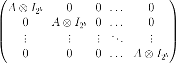
tensormatrix1
And each copy of $ A \otimes I_{2^b}$ looks like
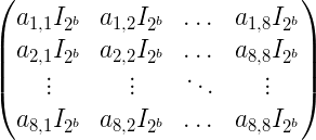
That’s a mess, but if you write it out for our example of swapping the first and third qubits of a three-qubit register you get the following:

example-3swap2
And this makes sense: the gate changes any entry of the state vector that has values for the first and third qubit that are different. This is what happens to our state:
$$\displaystyle v = \frac{1}{\sqrt{14}} (0,1,0,2,0,-3,0,0) \mapsto \frac{1}{\sqrt{14}} (0,0,0,0,1,-3,2,0)$$Perspective 2: just assume every operation works on the first three qubits, and wrap each operation $ A$ in between an operation that swaps the first three qubits with the desired three. So like $ BAB$ for $ B$ a swap operation. Then the matrix form looks a bit simpler, and it just means we permute the columns of the matrix form we gave above so that it just has the form $ A \otimes I_a$. This allows one to retain a shred of sanity when trying to envision the matrix for an operation that acts on three qubits that are not sequential. The downside is that to actually use this perspective in an analysis you have to carry around the extra baggage of these permutation matrices. So one might use this as a simplifying assumption (a “without loss of generality” statement).
Perspective 3: ignore matrices and write things down in a summation form. So if $ \sigma$ is the permutation that swaps 1 and 3 and leaves the other indices unchanged, we can write the general operation on a state $ v = \sum_{x \in \{ 0,1 \}^n } a_x e_{x}$ as $ Av = \sum_{x \in \{ 0,1 \}^n} a_x e_{\sigma(x)}$.
The third option is probably the nicest way to do things, but it’s important to keep the matrix view in mind for many reasons. Just one quick reason: “errors” in quantum gates (that are meant to approximately compute something) compound linearly in the number of gates because the operations are linear. This is a key reason that allows one to design quantum analogues of error correcting codes.
So we’ve established that the basic (atomic) quantum gates are “local” in the sense that they operate on a fixed number of qubits, but they are not local in the sense that they can screw up the entire state vector.
A side note on the meaning of “local”
When I was chugging through learning this stuff (and I still have far to go), I wanted to come up with an alternate characterization of the word “local” so that I would feel better about using the word “local.” Mathematicians are as passionate about word choice as programmers are about text editors. In particular, for a long time I was ignorantly convinced that quantum gates that act on a small number of qubits don’t affect the marginal distribution of measurement outcomes for other qubits. That is, I thought that if $ A$ acts on qubits 1,2,3, then $ Av$ and $ v$ have the same probability of a measurement producing a 1 in index 4, 5, etc, conditioned on fixing a measurement outcome for qubits 1,2,3. In notation, if $ x$ is a random variable whose values are binary strings and $ v$ is a state vector, I’ll call $ x \sim v$ the random process of measuring a state vector $ v$ and getting a string $ x$, then my claim was that the following was true for every $ b_1, b_2, b_3 \in \{0,1\}$ and every $ 1 \leq i \leq n$:
$$\displaystyle \begin{aligned}\Pr_{x \sim v}&[x_i = 1 \mid x_1 = b_1, x_2 = b_2, x_3 = b_3] = \\\ \Pr_{x \sim Av}&[x_i = 1 \mid x_1 = b_1, x_2 = b_2, x_3 = b_3] \end{aligned}$$You could try to prove this, and you would fail because it’s false. In fact, it’s even false if $ A$ acts on only a single qubit! Because it’s so tedious to write out all of the notation, I decided to write a program to illustrate the counterexample. (The most brazenly dedicated readers will try to prove this false fact and identify where the proof fails.)
import numpy

H = (1/(2**0.5)) * numpy.array([[1,1], [1,-1]])
I = numpy.identity(4)
A = numpy.kron(H,I)
Here $ H$ is the 2 by 2 Hadamard matrix, which operates on a single qubit and maps $ e_0 \mapsto \frac{e_0 + e_1}{\sqrt{2}}$, and $ e_1 \mapsto \frac{e_0 – e_1}{\sqrt{2}}$. This matrix is famous for many reasons, but one simple use as a quantum gate is to generate uniform random coin flips. In particular, measuring $ He_0$ outputs 1 and 0 with equal probability.
So in the code sample above, $ A$ is the mapping which applies the Hadamard operation to the first qubit and leaves the other qubits alone.
Then we compute some arbitrary input state vector $ w$
def normalize(z):
   return (1.0 / (sum(abs(z)**2) ** 0.5)) * z

v = numpy.arange(1,9)
w = normalize(v)
And now we write a function to compute the probability of some query conditioned on some fixed bits. We simply sum up the square norms of all of the relevant indices in the state vector.
def condProb(state, query={}, fixed={}):
   num = 0
   denom = 0
   dim = int(math.log2(len(state)))

   for x in itertools.product([0,1], repeat=dim):
      if any(x[index] != b for (index,b) in fixed.items()):
         continue

      i = sum(d << i for (i,d) in enumerate(reversed(x)))
      denom += abs(state[i])**2
      if all(x[index] == b for (index, b) in query.items()):
         num += abs(state[i]) ** 2

   if num == 0:
      return 0

   return num / denom
So if the query is query = {1:0} and the fixed thing is fixed = {0:0}, then this will compute the probability that the measurement results in the second qubit being zero conditioned on the first qubit also being zero.
And the result:
Aw = A.dot(w)
query = {1:0}
fixed = {0:0}
print((condProb(w, query, fixed), condProb(Aw, query, fixed)))
# (0.16666666666666666, 0.29069767441860467)
So they are not equal in general.
Also, in general we won’t work explicitly with full quantum gate matrices, since for $ n$ qubits the have size $ 2^{2n}$ which is big. But for finding counterexamples to guesses and false intuition, it’s a great tool.
Some important gates on 1-3 qubits
Let’s close this post with concrete examples of quantum gates. Based on the above discussion, we can write out the 2 x 2 or 4 x 4 matrix form of the operation and understand that it can apply to any two qubits in the state of a quantum program. Gates are most interesting when they’re operating on entangled qubits, and that will come out when we visit our first quantum algorithm next time, but for now we will just discuss at a naive level how they operate on the basis vectors.
Hadamard gate:
We introduced the Hadamard gate already, but I’ll reiterate it here.
Let $ H$ be the following 2 by 2 matrix, which operates on a single qubit and maps $ e_0 \mapsto \frac{e_0 + e_1}{\sqrt{2}}$, and $ e_1 \mapsto \frac{e_0 – e_1}{\sqrt{2}}$.
$$\displaystyle H = \frac{1}{\sqrt{2}} \begin{pmatrix} 1 & 1 \\\ 1 & -1 \end{pmatrix}$$One can use $ H$ to generate uniform random coin flips. In particular, measuring $ He_0$ outputs 1 and 0 with equal probability.
Quantum NOT gate:
Let $ X$ be the 2 x 2 matrix formed by swapping the columns of the identity matrix.
$$\displaystyle X = \begin{pmatrix} 0 & 1 \\\ 1 & 0 \end{pmatrix}$$This gate is often called the “Pauli-X” gate by physicists. This matrix is far too simple to be named after a person, and I can only imagine it is still named after a person for the layer of obfuscation that so often makes people feel smarter (same goes for the Pauli-Y and Pauli-Z gates, but we’ll get to those when we need them).
If we’re thinking of $ e_0$ as the boolean value “false” and $ e_1$ as the boolean value “true”, then the quantum NOT gate simply swaps those two states. In particular, note that composing a Hadamard and a quantum NOT gate can have interesting effects: $ XH(e_0) = H(e_0)$, but $ XH(e_1) \neq H(e_1)$. In the second case, the minus sign is the culprit. Which brings us to…
Phase shift gate:
Given an angle $ \theta$, we can “shift the phase” of one qubit by an angle of $ \theta$ using the 2 x 2 matrix $ R_{\theta}$.
$$\displaystyle R_{\theta} = \begin{pmatrix} 1 & 0 \\\ 0 & e^{i \theta} \end{pmatrix}$$“Phase” is a term physicists like to use for angles. Since the coefficients of a quantum state vector are complex numbers, and since complex numbers can be thought of geometrically as vectors with direction and magnitude, it makes sense to “rotate” the coefficient of a single qubit. So $ R_{\theta}$ does nothing to $ e_0$ and it rotates the coefficient of $ e_1$ by an angle of $ \theta$.
Continuing in our theme of concreteness, if I have the state vector $ v = \frac{1}{\sqrt{204}} (1,2,3,4,5,6,7,8)$ and I apply a rotation of $ pi$ to the second qubit, then my operation is the matrix $ I_2 \otimes R_{\pi} \otimes I_2$ which maps $ e_{i0k} \mapsto e_{i0k}$ and $ e_{i1k} \mapsto -e_{i1k}$. That would map the state $ v$ to $ (1,2,-3,-4,5,6,-7,-8)$.
If we instead used the rotation by $ \pi/2$ we would get the output state $ (1,2,3i, 4i, 5, 6, 7i, 8i)$.
Quantum AND/OR gate:
In the last post in this series we gave the quantum AND gate and left the quantum OR gate as an exercise. Rather than write out the matrix again, let me remind you of this gate using a description of the effect on the basis $ e_{ijk}$ where $ i,j,k \in \{ 0,1 \}$. Recall that we need three qubits in order to make the operation reversible (which is a consequence of all unitary gates being unitary matrices). Some notation: $ \oplus$ is the XOR of two bits, and $ \wedge$ is AND, $ \vee$ is OR. The quantum AND gate maps
$$\displaystyle e_{ijk} \mapsto e_{ij(k \oplus (i \wedge j))}$$In words, the third coordinate is XORed with the AND of the first two coordinates. We think of the third coordinate as a “scratchwork” qubit which is maybe prepared ahead of time to be in state zero.
Simiarly, the quantum OR gate maps $ e_{ijk} \mapsto e_{ij(k \oplus (i \vee j))}$. As we saw last time these combined with the quantum NOT gate (and some modest number of scratchwork qubits) allows quantum circuits to simulate any classical circuit.
Controlled-* gate:
The last example in this post is a meta-gate that represents a conditional branching. If we’re given a gate $ A$ acting on $ k$ qubits, then we define the controlled-A to be an operation which acts on $ k+1$ qubits. Let’s call the added qubit “qubit zero.” Then controlled-A does nothing if qubit zero is in state 0, and applies $ A$ if qubit zero is in state 1. Qubit zero is generally called the “control qubit.”
The matrix representing this operation decomposes into blocks if the control qubit is actually the first qubit (or you rearrange).
$$\displaystyle \begin{pmatrix} I_{2^{k-1}} & 0 \\\ 0 & A \end{pmatrix}$$A common example of this is the controlled-NOT gate, often abbreviated CNOT, and it has the matrix
$$\displaystyle \begin{pmatrix} 1 & 0 & 0 & 0 \\\ 0 & 1 & 0 & 0 \\\ 0 & 0 & 0 & 1 \\\ 0 & 0 & 1 & 0 \end{pmatrix}$$Looking forward
Okay let’s take a step back and evaluate our life choices. So far we’ve spent a few hours of our time motivating quantum computing, explaining the details of qubits and quantum circuits, and seeing examples of concrete quantum gates and studying measurement. I’ve hopefully hammered into your head the notion that quantum states which aren’t pure tensors (i.e. entangled) are where the “weirdness” of quantum computing comes from. But we haven’t seen any examples of quantum algorithms yet!
Next time we’ll see our first example of an algorithm that is genuinely quantum. We won’t tackle factoring yet, but we will see quantum “weirdness” in action.
Until then!
Want to respond? Send me an email, post a webmention, or find me elsewhere on the internet.