Data is abundant, data is big, and big is a problem. Let me start with an example. Let’s say you have a list of movie titles and you want to learn their genre: romance, action, drama, etc. And maybe in this scenario IMDB doesn’t exist so you can’t scrape the answer. Well, the title alone is almost never enough information. One nice way to get more data is to do the following:
- Pick a large dictionary of words, say the most common 100,000 non stop-words in the English language.
- Crawl the web looking for documents that include the title of a film.
- For each film, record the counts of all other words appearing in those documents.
- Maybe remove instances of “movie” or “film,” etc.
After this process you have a length-100,000 vector of integers associated with each movie title. IMDB’s database has around 1.5 million listed movies, and if we have a 32-bit integer per vector entry, that’s 600 GB of data to get every movie.
One way to try to find genres is to cluster this (unlabeled) dataset of vectors, and then manually inspect the clusters and assign genres. With a really fast computer we could simply run an existing clustering algorithm on this dataset and be done. Of course, clustering 600 GB of data takes a long time, but there’s another problem. The geometric intuition that we use to design clustering algorithms degrades as the length of the vectors in the dataset grows. As a result, our algorithms perform poorly. This phenomenon is called the “curse of dimensionality” (“curse” isn’t a technical term), and we’ll return to the mathematical curiosities shortly.
A possible workaround is to try to come up with faster algorithms or be more patient. But a more interesting mathematical question is the following:
Is it possible to condense high-dimensional data into smaller dimensions and retain the important geometric properties of the data?
This goal is called dimension reduction. Indeed, all of the chatter on the internet is bound to encode redundant information, so for our movie title vectors it seems the answer should be “yes.” But the questions remain, how does one find a low-dimensional condensification? (Condensification isn’t a word, the right word is embedding, but embedding is overloaded so we’ll wait until we define it) And what mathematical guarantees can you prove about the resulting condensed data? After all, it stands to reason that different techniques preserve different aspects of the data. Only math will tell.
In this post we’ll explore this so-called “curse” of dimensionality, explain the formality of why it’s seen as a curse, and implement a wonderfully simple technique called “the random projection method” which preserves pairwise distances between points after the reduction. As usual, and all the code, data, and tests used in the making of this post are on Github.
Some curious issues, and the “curse”
We start by exploring the curse of dimensionality with experiments on synthetic data.
In two dimensions, take a circle centered at the origin with radius 1 and its bounding square.
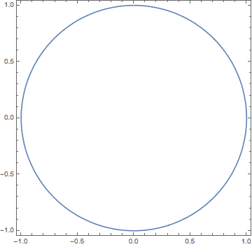
The circle fills up most of the area in the square, in fact it takes up exactly $ \pi$ out of 4 which is about 78%. In three dimensions we have a sphere and a cube, and the ratio of sphere volume to cube volume is a bit smaller, $ 4 \pi /3$ out of a total of 8, which is just over 52%. What about in a thousand dimensions? Let’s try by simulation.
import random

def randUnitCube(n):
   return [(random.random() - 0.5)*2 for _ in range(n)]

def sphereCubeRatio(n, numSamples):
   randomSample = [randUnitCube(n) for _ in range(numSamples)]
   return sum(1 for x in randomSample if sum(a**2 for a in x) <= 1) / numSamples
The result is as we computed for small dimension,
 >>> sphereCubeRatio(2,10000)
0.7857
>>> sphereCubeRatio(3,10000)
0.5196
And much smaller for larger dimension
>>> sphereCubeRatio(20,100000) # 100k samples
0.0
>>> sphereCubeRatio(20,1000000) # 1M samples
0.0
>>> sphereCubeRatio(20,2000000)
5e-07
Forget a thousand dimensions, for even twenty dimensions, a million samples wasn’t enough to register a single random point inside the unit sphere. This illustrates one concern, that when we’re sampling random points in the $ d$-dimensional unit cube, we need at least $ 2^d$ samples to ensure we’re getting a even distribution from the whole space. In high dimensions, this face basically rules out a naive Monte Carlo approximation, where you sample random points to estimate the probability of an event too complicated to sample from directly. A machine learning viewpoint of the same problem is that in dimension $ d$, if your machine learning algorithm requires a representative sample of the input space in order to make a useful inference, then you require $ 2^d$ samples to learn.
Luckily, we can answer our original question because there is a known formula for the volume of a sphere in any dimension. Rather than give the closed form formula, which involves the gamma function and is incredibly hard to parse, we’ll state the recursive form. Call $ V_i$ the volume of the unit sphere in dimension $ i$. Then $ V_0 = 1$ by convention, $ V_1 = 2$ (it’s an interval), and $ V_n = \frac{2 \pi V_{n-2}}{n}$. If you unpack this recursion you can see that the numerator looks like $ (2\pi)^{n/2}$ and the denominator looks like a factorial, except it skips every other number. So an even dimension would look like $ 2 \cdot 4 \cdot \dots \cdot n$, and this grows larger than a fixed exponential. So in fact the total volume of the sphere vanishes as the dimension grows! (In addition to the ratio vanishing!)
def sphereVolume(n):
   values = [0] * (n+1)
   for i in range(n+1):
      if i == 0:
         values[i] = 1
      elif i == 1:
         values[i] = 2
      else:
         values[i] = 2*math.pi / i * values[i-2]

   return values[-1]
This should be counterintuitive. I think most people would guess, when asked about how the volume of the unit sphere changes as the dimension grows, that it stays the same or gets bigger. But at a hundred dimensions, the volume is already getting too small to fit in a float.
>>> sphereVolume(20)
0.025806891390014047
>>> sphereVolume(100)
2.3682021018828297e-40
>>> sphereVolume(1000)
0.0
The scary thing is not just that this value drops, but that it drops exponentially quickly. A consequence is that, if you’re trying to cluster data points by looking at points within a fixed distance $ r$ of one point, you have to carefully measure how big $ r$ needs to be to cover the same proportional volume as it would in low dimension.
Here’s a related issue. Say I take a bunch of points generated uniformly at random in the unit cube.
from itertools import combinations

def distancesRandomPoints(n, numSamples):
   randomSample = [randUnitCube(n) for _ in range(numSamples)]
   pairwiseDistances = [dist(x,y) for (x,y) in combinations(randomSample, 2)]
   return pairwiseDistances
In two dimensions, the histogram of distances between points looks like this
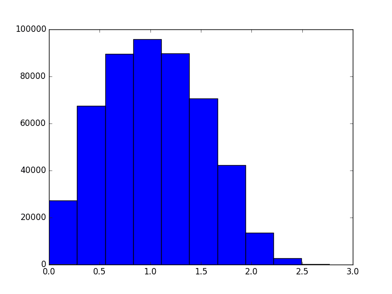
However, as the dimension grows the distribution of distances changes. It evolves like the following animation, in which each frame is an increase in dimension from 2 to 100.
The shape of the distribution doesn’t appear to be changing all that much after the first few frames, but the center of the distribution tends to infinity (in fact, it grows like $ \sqrt{n}$). The variance also appears to stay constant. This chart also becomes more variable as the dimension grows, again because we should be sampling exponentially many more points as the dimension grows (but we don’t). In other words, as the dimension grows the average distance grows and the tightness of the distribution stays the same. So at a thousand dimensions the average distance is about 26, tightly concentrated between 24 and 28. When the average is a thousand, the distribution is tight between 998 and 1002. If one were to normalize this data, it would appear that random points are all becoming equidistant from each other.
So in addition to the issues of runtime and sampling, the geometry of high-dimensional space looks different from what we expect. To get a better understanding of “big data,” we have to update our intuition from low-dimensional geometry with analysis and mathematical theorems that are much harder to visualize.
The Johnson-Lindenstrauss Lemma
Now we turn to proving dimension reduction is possible. There are a few methods one might first think of, such as look for suitable subsets of coordinates, or sums of subsets, but these would all appear to take a long time or they simply don’t work.
Instead, the key technique is to take a random linear subspace of a certain dimension, and project every data point onto that subspace. No searching required. The fact that this works is called the Johnson-Lindenstrauss Lemma. To set up some notation, we’ll call $ d(v,w)$ the usual distance between two points.
Lemma [Johnson-Lindenstrauss (1984)]: Given a set $ X$ of $ n$ points in $ \mathbb{R}^d$, project the points in $ X$ to a randomly chosen subspace of dimension $ c$. Call the projection $ \rho$. For any $ \varepsilon > 0$, if $ c$ is at least $ \Omega(\log(n) / \varepsilon^2)$, then with probability at least 1/2 the distances between points in $ X$ are preserved up to a factor of $ (1+\varepsilon)$. That is, with good probability every pair $ v,w \in X$ will satisfy
$$\displaystyle \| v-w \|^2 (1-\varepsilon) \leq \| \rho(v) – \rho(w) \|^2 \leq \| v-w \|^2 (1+\varepsilon)$$Before we do the proof, which is quite short, it’s important to point out that the target dimension $ c$ does not depend on the original dimension! It only depends on the number of points in the dataset, and logarithmically so. That makes this lemma seem like pure magic, that you can take data in an arbitrarily high dimension and put it in a much smaller dimension.
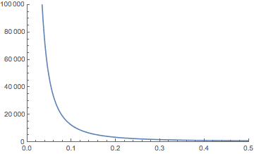
On the other hand, if you include all of the hidden constants in the bound on the dimension, it’s not that impressive. If your data have a million dimensions and you want to preserve the distances up to 1% ($ \varepsilon = 0.01$), the bound is bigger than a million! If you decrease the preservation $ \varepsilon$ to 10% (0.1), then you get down to about 12,000 dimensions, which is more reasonable. At 45% the bound drops to around 1,000 dimensions. Here’s a plot showing the theoretical bound on $ c$ in terms of $ \varepsilon$ for $ n$ fixed to a million.
But keep in mind, this is just a theoretical bound for potentially misbehaving data. Later in this post we’ll see if the practical dimension can be reduced more than the theory allows. As we’ll see, an algorithm run on the projected data is still effective even if the projection goes well beyond the theoretical bound. Because the theorem is known to be tight in the worst case (see the notes at the end) this speaks more to the robustness of the typical algorithm than to the robustness of the projection method.
A second important note is that this technique does not necessarily avoid all the problems with the curse of dimensionality. We mentioned above that one potential problem is that “random points” are roughly equidistant in high dimensions. Johnson-Lindenstrauss actually preserves this problem because it preserves distances! As a consequence, you won’t see strictly better algorithm performance if you project (which we suggested is possible in the beginning of this post). But you will alleviate slow runtimes if the runtime depends exponentially on the dimension. Indeed, if you replace the dimension $ d$ with the logarithm of the number of points $ \log n$, then $ 2^d$ becomes linear in $ n$, and $ 2^{O(d)}$ becomes polynomial.
Proof of the J-L lemma
Let’s prove the lemma.
Proof. To start we make note that one can sample from the uniform distribution on dimension-$ c$ linear subspaces of $ \mathbb{R}^d$ by choosing the entries of a $ c \times d$ matrix $ A$ independently from a normal distribution with mean 0 and variance 1. Then, to project a vector $ x$ by this matrix (call the projection $ \rho$), we can compute
$$\displaystyle \rho(x) = \frac{1}{\sqrt{c}}A x$$Now fix $ \varepsilon > 0$ and fix two points in the dataset $ x,y$. We want an upper bound on the probability that the following is false
$$\displaystyle \| x-y \|^2 (1-\varepsilon) \leq \| \rho(x) – \rho(y) \|^2 \leq \| x-y \|^2 (1+\varepsilon)$$Since that expression is a pain to work with, let’s rearrange it by calling $ u = x-y$, and rearranging (using the linearity of the projection) to get the equivalent statement.
$$\left | \| \rho(u) \|^2 – \|u \|^2 \right | \leq \varepsilon \| u \|^2$$And so we want a bound on the probability that this event does not occur, meaning the inequality switches directions.
Once we get such a bound (it will depend on $ c$ and $ \varepsilon$) we need to ensure that this bound is true for every pair of points. The union bound allows us to do this, but it also requires that the probability of the bad thing happening tends to zero faster than $ 1/\binom{n}{2}$. That’s where the $ \log(n)$ will come into the bound as stated in the theorem.
Continuing with our use of $ u$ for notation, define $ X$ to be the random variable $ \frac{c}{\| u \|^2} \| \rho(u) \|^2$. By expanding the notation and using the linearity of expectation, you can show that the expected value of $ X$ is $ c$, meaning that in expectation, distances are preserved. We are on the right track, and just need to show that the distribution of $ X$, and thus the possible deviations in distances, is tightly concentrated around $ c$. In full rigor, we will show
$$\displaystyle \Pr [X \geq (1+\varepsilon) c] < e^{-(\varepsilon^2 – \varepsilon^3) \frac{c}{4}}$$Let $ A_i$ denote the $ i$-th column of $ A$. Define by $ X_i$ the quantity $ \langle A_i, u \rangle / \| u \|$. This is a weighted average of the entries of $ A_i$ by the entries of $ u$. But since we chose the entries of $ A$ from the normal distribution, and since a weighted average of normally distributed random variables is also normally distributed (has the same distribution), $ X_i$ is a $ N(0,1)$ random variable. Moreover, each column is independent. This allows us to decompose $ X$ as
$$X = \frac{k}{\| u \|^2} \| \rho(u) \|^2 = \frac{\| Au \|^2}{\| u \|^2}$$Expanding further,
$$X = \sum_{i=1}^c \frac{\| A_i u \|^2}{\|u\|^2} = \sum_{i=1}^c X_i^2$$Now the event $ X \leq (1+\varepsilon) c$ can be expressed in terms of the nonegative variable $ e^{\lambda X}$, where $ 0 < \lambda < 1/2$ is parameter, to get
$$\displaystyle \Pr[X \geq (1+\varepsilon) c] = \Pr[e^{\lambda X} \geq e^{(1+\varepsilon)c \lambda}]$$This will become useful because the sum $ X = \sum_i X_i^2$ will split into a product momentarily. First we apply Markov’s inequality, which says that for any nonnegative random variable $ Y$, $ \Pr[Y \geq t] \leq \mathbb{E}[Y] / t$. This lets us write
$$\displaystyle \Pr[e^{\lambda X} \geq e^{(1+\varepsilon) c \lambda}] \leq \frac{\mathbb{E}[e^{\lambda X}]}{e^{(1+\varepsilon) c \lambda}}$$Now we can split up the exponent $ \lambda X$ into $ \sum_{i=1}^c \lambda X_i^2$, and using the i.i.d.-ness of the $ X_i^2$ we can rewrite the RHS of the inequality as
$$\left ( \frac{\mathbb{E}[e^{\lambda X_1^2}]}{e^{(1+\varepsilon)\lambda}} \right )^c$$A similar statement using $ -\lambda$ is true for the $ (1-\varepsilon)$ part, namely that
$$\displaystyle \Pr[X \leq (1-\varepsilon)c] \leq \left ( \frac{\mathbb{E}[e^{-\lambda X_1^2}]}{e^{-(1-\varepsilon)\lambda}} \right )^c$$The last thing that’s needed is to bound $ \mathbb{E}[e^{\lambda X_i^2}]$, but since $ X_i^2 \sim N(0,1)$, we can use the known density function for a normal distribution, and integrate to get the exact value $ \mathbb{E}[e^{\lambda X_1^2}] = \frac{1}{\sqrt{1-2\lambda}}$. Including this in the bound gives us a closed-form bound in terms of $ \lambda, c, \varepsilon$. Using standard calculus the optimal $ \lambda \in (0,1/2)$ is $ \lambda = \varepsilon / 2(1+\varepsilon)$. This gives
$$\displaystyle \Pr[X \geq (1+\varepsilon) c] \leq ((1+\varepsilon)e^{-\varepsilon})^{c/2}$$Using the Taylor series expansion for $ e^x$, one can show the bound $ 1+\varepsilon < e^{\varepsilon – (\varepsilon^2 – \varepsilon^3)/2}$, which simplifies the final upper bound to $ e^{-(\varepsilon^2 – \varepsilon^3) c/4}$.
Doing the same thing for the $ (1-\varepsilon)$ version gives an equivalent bound, and so the total bound is doubled, i.e. $ 2e^{-(\varepsilon^2 – \varepsilon^3) c/4}$.
As we said at the beginning, applying the union bound means we need
$$\displaystyle 2e^{-(\varepsilon^2 – \varepsilon^3) c/4} < \frac{1}{\binom{n}{2}}$$Solving this for $ c$ gives $ c \geq \frac{8 \log m}{\varepsilon^2 – \varepsilon^3}$, as desired.
$$\square$$Projecting in Practice
Let’s write a python program to actually perform the Johnson-Lindenstrauss dimension reduction scheme. This is sometimes called the Johnson-Lindenstrauss transform, or JLT.
First we define a random subspace by sampling an appropriately-sized matrix with normally distributed entries, and a function that performs the projection onto a given subspace (for testing).
import random
import math
import numpy

def randomSubspace(subspaceDimension, ambientDimension):
   return numpy.random.normal(0, 1, size=(subspaceDimension, ambientDimension))

def project(v, subspace):
   subspaceDimension = len(subspace)
   return (1 / math.sqrt(subspaceDimension)) * subspace.dot(v)
We have a function that computes the theoretical bound on the optimal dimension to reduce to.
def theoreticalBound(n, epsilon):
   return math.ceil(8*math.log(n) / (epsilon**2 - epsilon**3))
And then performing the JLT is simply matrix multiplication
def jlt(data, subspaceDimension):
   ambientDimension = len(data[0])
   A = randomSubspace(subspaceDimension, ambientDimension)
   return (1 / math.sqrt(subspaceDimension)) * A.dot(data.T).T
The high-dimensional dataset we’ll use comes from a data mining competition called KDD Cup 2001. The dataset we used deals with drug design, and the goal is to determine whether an organic compound binds to something called thrombin. Thrombin has something to do with blood clotting, and I won’t pretend I’m an expert. The dataset, however, has over a hundred thousand features for about 2,000 compounds. Here are a few approximate target dimensions we can hope for as epsilon varies.
>>> [((1/x),theoreticalBound(n=2000, epsilon=1/x))
       for x in [2, 3, 4, 5, 6, 7, 8, 9, 10, 15, 20]]
[('0.50', 487), ('0.33', 821), ('0.25', 1298), ('0.20', 1901),
 ('0.17', 2627), ('0.14', 3477), ('0.12', 4448), ('0.11', 5542),
 ('0.10', 6757), ('0.07', 14659), ('0.05', 25604)]
Going down from a hundred thousand dimensions to a few thousand is by any measure decreases the size of the dataset by about 95%. We can also observe how the distribution of overall distances varies as the size of the subspace we project to varies.
The animation proceeds from 5000 dimensions down to 2 (when the plot is at its bulkiest closer to zero).
The last three frames are for 10, 5, and 2 dimensions respectively. As you can see the histogram starts to beef up around zero. To be honest I was expecting something a bit more dramatic like a uniform-ish distribution. Of course, the distribution of distances is not all that matters. Another concern is the worst case change in distances between any two points before and after the projection. We can see that indeed when we project to the dimension specified in the theorem, that the distances are within the prescribed bounds.
def checkTheorem(oldData, newData, epsilon):
   numBadPoints = 0

   for (x,y), (x2,y2) in zip(combinations(oldData, 2), combinations(newData, 2)):
      oldNorm = numpy.linalg.norm(x2-y2)**2
      newNorm = numpy.linalg.norm(x-y)**2

      if newNorm == 0 or oldNorm == 0:
         continue

      if abs(oldNorm / newNorm - 1) > epsilon:
         numBadPoints += 1

   return numBadPoints

if __name__ == "__main__"
   from data import thrombin
   train, labels = thrombin.load()

   numPoints = len(train)
   epsilon = 0.2
   subspaceDim = theoreticalBound(numPoints, epsilon)
   ambientDim = len(train[0])
   newData = jlt(train, subspaceDim)

   print(checkTheorem(train, newData, epsilon))
This program prints zero every time I try running it, which is the poor man’s way of saying it works “with high probability.” We can also plot statistics about the number of pairs of data points that are distorted by more than $ \varepsilon$ as the subspace dimension shrinks. We ran this on the following set of subspace dimensions with $ \varepsilon = 0.1$ and took average/standard deviation over twenty trials:
dims = [1000, 750, 500, 250, 100, 75, 50, 25, 10, 5, 2]
The result is the following chart, whose x-axis is the dimension projected to (so the left hand is the most extreme projection to 2, 5, 10 dimensions), the y-axis is the number of distorted pairs, and the error bars represent a single standard deviation away from the mean.
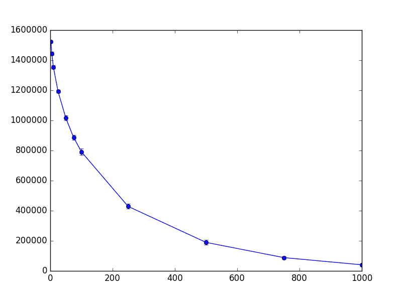
thrombin-worst-case
This chart provides good news about this dataset because the standard deviations are low. It tells us something that mathematicians often ignore: the predictability of the tradeoff that occurs once you go past the theoretically perfect bound. In this case, the standard deviations tell us that it’s highly predictable. Moreover, since this tradeoff curve measures pairs of points, we might conjecture that the distortion is localized around a single set of points that got significantly “rattled” by the projection. This would be an interesting exercise to explore.
Now all of these charts are really playing with the JLT and confirming the correctness of our code (and hopefully our intuition). The real question is: how well does a machine learning algorithm perform on the original data when compared to the projected data? If the algorithm only “depends” on the pairwise distances between the points, then we should expect nearly identical accuracy in the unprojected and projected versions of the data. To show this we’ll use an easy learning algorithm, the k-nearest-neighbors clustering method. The problem, however, is that there are very few positive examples in this particular dataset. So looking for the majority label of the nearest $ k$ neighbors for any $ k > 2$ unilaterally results in the “all negative” classifier, which has 97% accuracy. This happens before and after projecting.
To compensate for this, we modify k-nearest-neighbors slightly by having the label of a predicted point be 1 if any label among its nearest neighbors is 1. So it’s not a majority vote, but rather a logical OR of the labels of nearby neighbors. Our point in this post is not to solve the problem well, but rather to show how an algorithm (even a not-so-good one) can degrade as one projects the data into smaller and smaller dimensions. Here is the code.
def nearestNeighborsAccuracy(data, labels, k=10):
   from sklearn.neighbors import NearestNeighbors
   trainData, trainLabels, testData, testLabels = randomSplit(data, labels) # cross validation
   model = NearestNeighbors(n_neighbors=k).fit(trainData)
   distances, indices = model.kneighbors(testData)
   predictedLabels = []

   for x in indices:
      xLabels = [trainLabels[i] for i in x[1:]]
      predictedLabel = max(xLabels)
      predictedLabels.append(predictedLabel)

   totalAccuracy = sum(x == y for (x,y) in zip(testLabels, predictedLabels)) / len(testLabels)
   falsePositive = (sum(x == 0 and y == 1 for (x,y) in zip(testLabels, predictedLabels)) /
      sum(x == 0 for x in testLabels))
   falseNegative = (sum(x == 1 and y == 0 for (x,y) in zip(testLabels, predictedLabels)) /
      sum(x == 1 for x in testLabels))

   return totalAccuracy, falsePositive, falseNegative
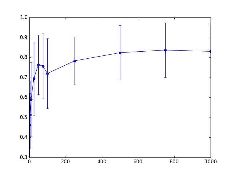
And here is the accuracy of this modified k-nearest-neighbors algorithm run on the thrombin dataset. The horizontal line represents the accuracy of the produced classifier on the unmodified data set. The x-axis represents the dimension projected to (left-hand side is the lowest), and the y-axis represents the accuracy. The mean accuracy over fifty trials was plotted, with error bars representing one standard deviation. The complete code to reproduce the plot is in the Github repository.
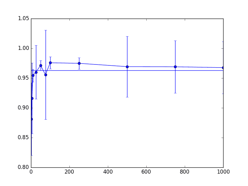
thrombin-knn-accuracy
Likewise, we plot the proportion of false positive and false negatives for the output classifier. Note that a “positive” label made up only about 2% of the total data set. First the false positives
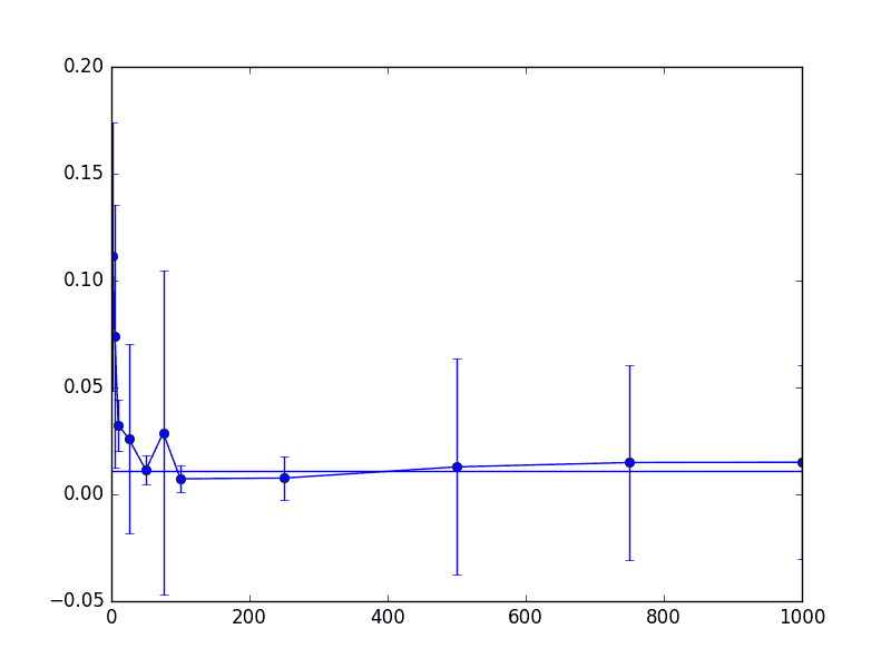
thrombin-knn-fp
Then the false negatives
thrombin-knn-fn
As we can see from these three charts, things don’t really change that much (for this dataset) even when we project down to around 200-300 dimensions. Note that for these parameters the “correct” theoretical choice for dimension was on the order of 5,000 dimensions, so this is a 95% savings from the naive approach, and 99.75% space savings from the original data. Not too shabby.
Notes
The $ \Omega(\log(n))$ worst-case dimension bound is asymptotically tight, though there is some small gap in the literature that depends on $ \varepsilon$. This result is due to Noga Alon, the very last result (Section 9) of this paper. [Update: as djhsu points out in the comments, this gap is now closed thanks to Larsen and Nelson]
We did dimension reduction with respect to preserving the Euclidean distance between points. One might naturally wonder if you can achieve the same dimension reduction with a different metric, say the taxicab metric or a $ p$-norm. In fact, you cannot achieve anything close to logarithmic dimension reduction for the taxicab ($ l_1$) metric. This result is due to Brinkman-Charikar in 2004.
The code we used to compute the JLT is not particularly efficient. There are much more efficient methods. One of them, borrowing its namesake from the Fast Fourier Transform, is called the Fast Johnson-Lindenstrauss Transform. The technique is due to Ailon-Chazelle from 2009, and it involves something called “preconditioning a sparse projection matrix with a randomized Fourier transform.” I don’t know precisely what that means, but it would be neat to dive into that in a future post.
The central focus in this post was whether the JLT preserves distances between points, but one might be curious as to whether the points themselves are well approximated. The answer is an enthusiastic no. If the data were images, the projected points would look nothing like the original images. However, it appears the degradation tradeoff is measurable (by some accounts perhaps linear), and there appears to be some work (also this by the same author) when restricting to sparse vectors (like word-association vectors).
Note that the JLT is not the only method for dimensionality reduction. We previously saw principal component analysis (applied to face recognition), and in the future we will cover a related technique called the Singular Value Decomposition. It is worth noting that another common technique specific to nearest-neighbor is called “locality-sensitive hashing.” Here the goal is to project the points in such a way that “similar” points land very close to each other. Say, if you were to discretize the plane into bins, these bins would form the hash values and you’d want to maximize the probability that two points with the same label land in the same bin. Then you can do things like nearest-neighbors by comparing bins.
Another interesting note, if your data is linearly separable (like the examples we saw in our age-old post on Perceptrons), then you can use the JLT to make finding a linear separator easier. First project the data onto the dimension given in the theorem. With high probability the points will still be linearly separable. And then you can use a perceptron-type algorithm in the smaller dimension. If you want to find out which side a new point is on, you project and compare with the separator in the smaller dimension.
Beyond its interest for practical dimensionality reduction, the JLT has had many other interesting theoretical consequences. More generally, the idea of “randomly projecting” your data onto some small dimensional space has allowed mathematicians to get some of the best-known results on many optimization and learning problems, perhaps the most famous of which is called MAX-CUT; the result is by Goemans-Williamson and it led to a mathematical constant being named after them, $ \alpha_{GW} =.878567 \dots$. If you’re interested in more about the theory, Santosh Vempala wrote a wonderful (and short!) treatise dedicated to this topic.
randomprojectionbook
Want to respond? Send me an email, post a webmention, or find me elsewhere on the internet.