
papad
Hard to believe
Sanjeev Arora and his coauthors consider it “a basic tool [that should be] taught to all algorithms students together with divide-and-conquer, dynamic programming, and random sampling.” Christos Papadimitriou calls it “so hard to believe that it has been discovered five times and forgotten.” It has formed the basis of algorithms in machine learning, optimization, game theory, economics, biology, and more.
What mystical algorithm has such broad applications? Now that computer scientists have studied it in generality, it’s known as the Multiplicative Weights Update Algorithm (MWUA). Procedurally, the algorithm is simple. I can even describe the core idea in six lines of pseudocode. You start with a collection of $ n$ objects, and each object has a weight.
Set all the object weights to be 1.
For some large number of rounds:
   Pick an object at random proportionally to the weights
   Some event happens
   Increase the weight of the chosen object if it does well in the event
   Otherwise decrease the weight
The name “multiplicative weights” comes from how we implement the last step: if the weight of the chosen object at step $ t$ is $ w_t$ before the event, and $ G$ represents how well the object did in the event, then we’ll update the weight according to the rule:
$$\displaystyle w_{t+1} = w_t (1 + G)$$Think of this as increasing the weight by a small multiple of the object’s performance on a given round.
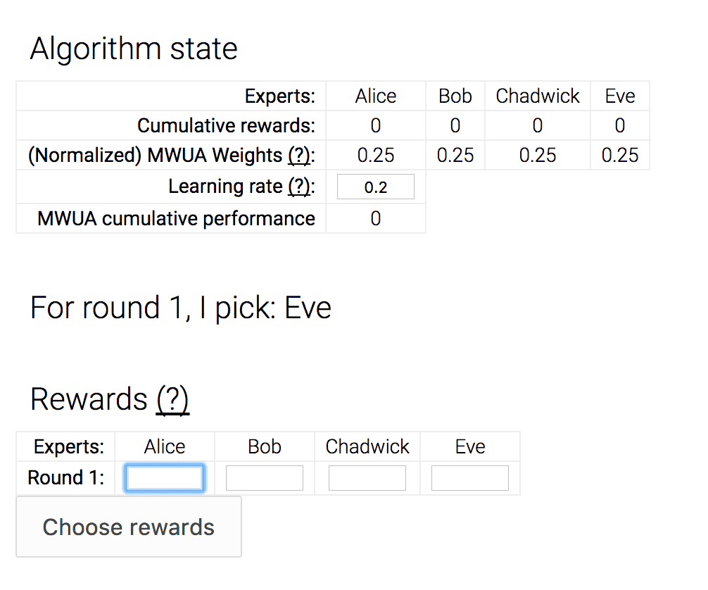
Here is a simple example of how it might be used. You have some money you want to invest, and you have a bunch of financial experts who are telling you what to invest in every day. So each day you pick an expert, and you follow their advice, and you either make a thousand dollars, or you lose a thousand dollars, or something in between. Then you repeat, and your goal is to figure out which expert is the most reliable.
This is how we use multiplicative weights: if we number the experts $ 1, \dots, N$, we give each expert a weight $ w_i$ which starts at 1. Then, each day we pick an expert at random (where experts with larger weights are more likely to be picked) and at the end of the day we have some gain or loss $ G$. Then we update the weight of the chosen expert by multiplying it by $ (1 + G / 1000)$. Sometimes you have enough information to update the weights of experts you didn’t choose, too. The theoretical guarantees of the algorithm say we’ll find the best expert quickly (“quickly” will be concrete later).
In fact, let’s play a game where you, dear reader, get to decide the rewards for each expert and each day. I programmed the multiplicative weights algorithm to react according to your choices. Click the image below to go to the demo.
mwua
This core mechanism of updating weights can be interpreted in many ways, and that’s part of the reason it has sprouted up all over mathematics and computer science. Just a few examples of where this has led:
- In game theory, weights are the “belief” of a player about the strategy of an opponent. The most famous algorithm to use this is called Fictitious Play, and others include EXP3 for minimizing regret in the so-called “adversarial bandit learning” problem.
- In machine learning, weights are the difficulty of a specific training example, so that higher weights mean the learning algorithm has to “try harder” to accommodate that example. The first result I’m aware of for this is the Perceptron (and similar Winnow) algorithm for learning hyperplane separators. The most famous is the AdaBoost algorithm.
- Analogously, in optimization, the weights are the difficulty of a specific constraint, and this technique can be used to approximately solve linear and semidefinite programs. The approximation is because MWUA only provides a solution with some error.
- In mathematical biology, the weights represent the fitness of individual alleles, and filtering reproductive success based on this and updating weights for successful organisms produces a mechanism very much like evolution. With modifications, it also provides a mechanism through which to understand sex in the context of evolutionary biology.
- The TCP protocol, which basically defined the internet, uses additive and multiplicative weight updates (which are very similar in the analysis) to manage congestion.
- You can get easy $ \log(n)$-approximation algorithms for many NP-hard problems, such as set cover.
Additional, more technical examples can be found in this survey of Arora et al.
In the rest of this post, we’ll implement a generic Multiplicative Weights Update Algorithm, we’ll prove it’s main theoretical guarantees, and we’ll implement a linear program solver as an example of its applicability. As usual, all of the code used in the making of this post is available in a Github repository.
The generic MWUA algorithm
Let’s start by writing down pseudocode and an implementation for the MWUA algorithm in full generality.
In general we have some set $ X$ of objects and some set $ Y$ of “event outcomes” which can be completely independent. If these sets are finite, we can write down a table $ M$ whose rows are objects, whose columns are outcomes, and whose $ i,j$ entry $ M(i,j)$ is the reward produced by object $ x_i$ when the outcome is $ y_j$. We will also write this as $ M(x, y)$ for object $ x$ and outcome $ y$. The only assumption we’ll make on the rewards is that the values $ M(x, y)$ are bounded by some small constant $ B$ (by small I mean $ B$ should not require exponentially many bits to write down as compared to the size of $ X$). In symbols, $ M(x,y) \in [0,B]$. There are minor modifications you can make to the algorithm if you want negative rewards, but for simplicity we will leave that out. Note the table $ M$ just exists for analysis, and the algorithm does not know its values. Moreover, while the values in $ M$ are static, the choice of outcome $ y$ for a given round may be nondeterministic.
The MWUA algorithm randomly chooses an object $ x \in X$ in every round, observing the outcome $ y \in Y$, and collecting the reward $ M(x,y)$ (or losing it as a penalty). The guarantee of the MWUA theorem is that the expected sum of rewards/penalties of MWUA is not much worse than if one had picked the best object (in hindsight) every single round.
Let’s describe the algorithm in notation first and build up pseudocode as we go. The input to the algorithm is the set of objects, a subroutine that observes an outcome, a black-box reward function, a learning rate parameter, and a number of rounds.
def MWUA(objects, observeOutcome, reward, learningRate, numRounds):
   ...
We define for object $ x$ a nonnegative number $ w_x$ we call a “weight.” The weights will change over time so we’ll also sub-script a weight with a round number $ t$, i.e. $ w_{x,t}$ is the weight of object $ x$ in round $ t$. Initially, all the weights are $ 1$. Then MWUA continues in rounds. We start each round by drawing an example randomly with probability proportional to the weights. Then we observe the outcome for that round and the reward for that round.
# draw: [float] -> int
# pick an index from the given list of floats proportionally
# to the size of the entry (i.e. normalize to a probability
# distribution and draw according to the probabilities).
def draw(weights):
    choice = random.uniform(0, sum(weights))
    choiceIndex = 0

    for weight in weights:
        choice -= weight
        if choice <= 0:
            return choiceIndex

        choiceIndex += 1

# MWUA: the multiplicative weights update algorithm
def MWUA(objects, observeOutcome, reward, learningRate numRounds):
   weights = [1] * len(objects)
   for t in numRounds:
      chosenObjectIndex = draw(weights)
      chosenObject = objects[chosenObjectIndex]

      outcome = observeOutcome(t, weights, chosenObject)
      thisRoundReward = reward(chosenObject, outcome)

      ...
Sampling objects in this way is the same as associating a distribution $ D_t$ to each round, where if $ S_t = \sum_{x \in X} w_{x,t}$ then the probability of drawing $ x$, which we denote $ D_t(x)$, is $ w_{x,t} / S_t$. We don’t need to keep track of this distribution in the actual run of the algorithm, but it will help us with the mathematical analysis.
Next comes the weight update step. Let’s call our learning rate variable parameter $ \varepsilon$. In round $ t$ say we have object $ x_t$ and outcome $ y_t$, then the reward is $ M(x_t, y_t)$. We update the weight of the chosen object $ x_t$ according to the formula:
$$\displaystyle w_{x_t, t} = w_{x_t} (1 + \varepsilon M(x_t, y_t) / B)$$In the more general event that you have rewards for all objects (if not, the reward-producing function can output zero), you would perform this weight update on all objects $ x \in X$. This turns into the following Python snippet, where we hide the division by $ B$ into the choice of learning rate:
# MWUA: the multiplicative weights update algorithm
def MWUA(objects, observeOutcome, reward, learningRate, numRounds):
   weights = [1] * len(objects)
   for t in numRounds:
      chosenObjectIndex = draw(weights)
      chosenObject = objects[chosenObjectIndex]

      outcome = observeOutcome(t, weights, chosenObject)
      thisRoundReward = reward(chosenObject, outcome)

      for i in range(len(weights)):
         weights[i] *= (1 + learningRate * reward(objects[i], outcome))
One of the amazing things about this algorithm is that the outcomes and rewards could be chosen adaptively by an adversary who knows everything about the MWUA algorithm (except which random numbers the algorithm generates to make its choices). This means that the rewards in round $ t$ can depend on the weights in that same round! We will exploit this when we solve linear programs later in this post.
But even in such an oppressive, exploitative environment, MWUA persists and achieves its guarantee. And now we can state that guarantee.
Theorem (from Arora et al): The cumulative reward of the MWUA algorithm is, up to constant multiplicative factors, at least the cumulative reward of the best object minus $ \log(n)$, where $ n$ is the number of objects. (Exact formula at the end of the proof)
The core of the proof, which we’ll state as a lemma, uses one of the most elegant proof techniques in all of mathematics. It’s the idea of constructing a potential function, and tracking the change in that potential function over time. Such a proof usually has the mysterious script:
- Define potential function, in our case $ S_t$.
- State what seems like trivial facts about the potential function to write $ S_{t+1}$ in terms of $ S_t$, and hence get general information about $ S_T$ for some large $ T$.
- Theorem is proved.
- Wait, what?
Clearly, coming up with a useful potential function is a difficult and prized skill.
In this proof our potential function is the sum of the weights of the objects in a given round, $ S_t = \sum_{x \in X} w_{x, t}$. Now the lemma.
Lemma: Let $ B$ be the bound on the size of the rewards, and $ 0 < \varepsilon < 1/2$ a learning parameter. Recall that $ D_t(x)$ is the probability that MWUA draws object $ x$ in round $ t$. Write the expected reward for MWUA for round $ t$ as the following (using only the definition of expected value):
$$\displaystyle R_t = \sum_{x \in X} D_t(x) M(x, y_t)$$Then the claim of the lemma is:
$$\displaystyle S_{t+1} \leq S_t e^{\varepsilon R_t / B}$$Proof. Expand $ S_{t+1} = \sum_{x \in X} w_{x, t+1}$ using the definition of the MWUA update:
$$\displaystyle \sum_{x \in X} w_{x, t+1} = \sum_{x \in X} w_{x, t}(1 + \varepsilon M(x, y_t) / B)$$Now distribute $ w_{x, t}$ and split into two sums:
$$\displaystyle \dots = \sum_{x \in X} w_{x, t} + \frac{\varepsilon}{B} \sum_{x \in X} w_{x,t} M(x, y_t)$$Using the fact that $ D_t(x) = \frac{w_{x,t}}{S_t}$, we can replace $ w_{x,t}$ with $ D_t(x) S_t$, which allows us to get $ R_t$
$$\displaystyle \begin{aligned} \dots &= S_t + \frac{\varepsilon S_t}{B} \sum_{x \in X} D_t(x) M(x, y_t) \\\ &= S_t \left ( 1 + \frac{\varepsilon R_t}{B} \right ) \end{aligned}$$And then using the fact that $ (1 + x) \leq e^x$ (Taylor series), we can bound the last expression by $ S_te^{\varepsilon R_t / B}$, as desired.
$$\square$$Now using the lemma, we can get a hold on $ S_T$ for a large $ T$, namely that
$$\displaystyle S_T \leq S_1 e^{\varepsilon \sum_{t=1}^T R_t / B}$$If $ |X| = n$ then $ S_1=n$, simplifying the above. Moreover, the sum of the weights in round $ T$ is certainly greater than any single weight, so that for every fixed object $ x \in X$,
$$\displaystyle S_T \geq w_{x,T} \leq (1 + \varepsilon)^{\sum_t M(x, y_t) / B}$$Squeezing $ S_t$ between these two inequalities and taking logarithms (to simplify the exponents) gives
$$\displaystyle \left ( \sum_t M(x, y_t) / B \right ) \log(1+\varepsilon) \leq \log n + \frac{\varepsilon}{B} \sum_t R_t$$Multiply through by $ B$, divide by $ \varepsilon$, rearrange, and use the fact that when $ 0 < \varepsilon < 1/2$ we have $ \log(1 + \varepsilon) \geq \varepsilon – \varepsilon^2$ (Taylor series) to get
$$\displaystyle \sum_t R_t \geq \left [ \sum_t M(x, y_t) \right ] (1-\varepsilon) – \frac{B \log n}{\varepsilon}$$The bracketed term is the payoff of object $ x$, and MWUA’s payoff is at least a fraction of that minus the logarithmic term. The bound applies to any object $ x \in X$, and hence to the best one. This proves the theorem.
$$\square$$Briefly discussing the bound itself, we see that the smaller the learning rate is, the closer you eventually get to the best object, but by contrast the more the subtracted quantity $ B \log(n) / \varepsilon$ hurts you. If your target is an absolute error bound against the best performing object on average, you can do more algebra to determine how many rounds you need in terms of a fixed $ \delta$. The answer is roughly: let $ \varepsilon = O(\delta / B)$ and pick $ T = O(B^2 \log(n) / \delta^2)$. See this survey for more.
MWUA for linear programs
Now we’ll approximately solve a linear program using MWUA. Recall that a linear program is an optimization problem whose goal is to minimize (or maximize) a linear function of many variables. The objective to minimize is usually given as a dot product $ c \cdot x$, where $ c$ is a fixed vector and $ x = (x_1, x_2, \dots, x_n)$ is a vector of non-negative variables the algorithm gets to choose. The choices for $ x$ are also constrained by a set of $ m$ linear inequalities, $ A_i \cdot x \geq b_i$, where $ A_i$ is a fixed vector and $ b_i$ is a scalar for $ i = 1, \dots, m$. This is usually summarized by putting all the $ A_i$ in a matrix, $ b_i$ in a vector, as
$$x_{\textup{OPT}} = \textup{argmin}_x \{ c \cdot x \mid Ax \geq b, x \geq 0 \}$$We can further simplify the constraints by assuming we know the optimal value $ Z = c \cdot x_{\textup{OPT}}$ in advance, by doing a binary search (more on this later). So, if we ignore the hard constraint $ Ax \geq b$, the “easy feasible region” of possible $ x$’s includes $ \{ x \mid x \geq 0, c \cdot x = Z \}$.
In order to fit linear programming into the MWUA framework we have to define two things.
- The objects: the set of linear inequalities $ A_i \cdot x \geq b_i$.
- The rewards: the error of a constraint for a special input vector $ x_t$.
Number 2 is curious (why would we give a reward for error?) but it’s crucial and we’ll discuss it momentarily.
The special input $ x_t$ depends on the weights in round $ t$ (which is allowed, recall). Specifically, if the weights are $ w = (w_1, \dots, w_m)$, we ask for a vector $ x_t$ in our “easy feasible region” which satisfies
$$\displaystyle (A^T w) \cdot x_t \geq w \cdot b$$For this post we call the implementation of procuring such a vector the “oracle,” since it can be seen as the black-box problem of, given a vector $ \alpha$ and a scalar $ \beta$ and a convex region $ R$, finding a vector $ x \in R$ satisfying $ \alpha \cdot x \geq \beta$. This allows one to solve more complex optimization problems with the same technique, swapping in a new oracle as needed. Our choice of inputs, $ \alpha = A^T w, \beta = w \cdot b$, are particular to the linear programming formulation.
Two remarks on this choice of inputs. First, the vector $ A^T w$ is a weighted average of the constraints in $ A$, and $ w \cdot b$ is a weighted average of the thresholds. So this this inequality is a “weighted average” inequality (specifically, a convex combination, since the weights are nonnegative). In particular, if no such $ x$ exists, then the original linear program has no solution. Indeed, given a solution $ x^*$ to the original linear program, each constraint, say $ A_1 x^*_1 \geq b_1$, is unaffected by left-multiplication by $ w_1$.
Second, and more important to the conceptual understanding of this algorithm, the choice of rewards and the multiplicative updates ensure that easier constraints show up less prominently in the inequality by having smaller weights. That is, if we end up overly satisfying a constraint, we penalize that object for future rounds so we don’t waste our effort on it. The byproduct of MWUA—the weights—identify the hardest constraints to satisfy, and so in each round we can put a proportionate amount of effort into solving (one of) the hard constraints. This is why it makes sense to reward error; the error is a signal for where to improve, and by over-representing the hard constraints, we force MWUA’s attention on them.
At the end, our final output is an average of the $ x_t$ produced in each round, i.e. $ x^* = \frac{1}{T}\sum_t x_t$. This vector satisfies all the constraints to a roughly equal degree. We will skip the proof that this vector does what we want, but see these notes for a simple proof. We’ll spend the rest of this post implementing the scheme outlined above.
Implementing the oracle
Fix the convex region $ R = \{ c \cdot x = Z, x \geq 0 \}$ for a known optimal value $ Z$. Define $ \textup{oracle}(\alpha, \beta)$ as the problem of finding an $ x \in R$ such that $ \alpha \cdot x \geq \beta$.
For the case of this linear region $ R$, we can simply find the index $ i$ which maximizes $ \alpha_i Z / c_i$. If this value exceeds $ \beta$, we can return the vector with that value in the $ i$-th position and zeros elsewhere. Otherwise, the problem has no solution.
To prove the “no solution” part, say $ n=2$ and you have $ x = (x_1, x_2)$ a solution to $ \alpha \cdot x \geq \beta$. Then for whichever index makes $ \alpha_i Z / c_i$ bigger, say $ i=1$, you can increase $ \alpha \cdot x$ without changing $ c \cdot x = Z$ by replacing $ x_1$ with $ x_1 + (c_2/c_1)x_2$ and $ x_2$ with zero. I.e., we’re moving the solution $ x$ along the line $ c \cdot x = Z$ until it reaches a vertex of the region bounded by $ c \cdot x = Z$ and $ x \geq 0$. This must happen when all entries but one are zero. This is the same reason why optimal solutions of (generic) linear programs occur at vertices of their feasible regions.
The code for this becomes quite simple. Note we use the numpy library in the entire codebase to make linear algebra operations fast and simple to read.
def makeOracle(c, optimalValue):
    n = len(c)

    def oracle(weightedVector, weightedThreshold):
        def quantity(i):
            return weightedVector[i] * optimalValue / c[i] if c[i] > 0 else -1

        biggest = max(range(n), key=quantity)
        if quantity(biggest) < weightedThreshold:
            raise InfeasibleException

        return numpy.array([optimalValue / c[i] if i == biggest else 0 for i in range(n)])

    return oracle
Implementing the core solver
The core solver implements the discussion from previously, given the optimal value of the linear program as input. To avoid too many single-letter variable names, we use linearObjective instead of $ c$.
def solveGivenOptimalValue(A, b, linearObjective, optimalValue, learningRate=0.1):
    m, n = A.shape  # m equations, n variables
    oracle = makeOracle(linearObjective, optimalValue)

    def reward(i, specialVector):
        ...

    def observeOutcome(_, weights, __):
        ...

    numRounds = 1000
    weights, cumulativeReward, outcomes = MWUA(
        range(m), observeOutcome, reward, learningRate, numRounds
    )
    averageVector = sum(outcomes) / numRounds

    return averageVector
First we make the oracle, then the reward and outcome-producing functions, then we invoke the MWUA subroutine. Here are those two functions; they are closures because they need access to $ A$ and $ b$. Note that neither $ c$ nor the optimal value show up here.
    def reward(i, specialVector):
        constraint = A[i]
        threshold = b[i]
        return threshold - numpy.dot(constraint, specialVector)

    def observeOutcome(_, weights, __):
        weights = numpy.array(weights)
        weightedVector = A.transpose().dot(weights)
        weightedThreshold = weights.dot(b)
        return oracle(weightedVector, weightedThreshold)
Implementing the binary search, and an example
Finally, the top-level routine. Note that the binary search for the optimal value is sophisticated (though it could be more sophisticated). It takes a max range for the search, and invokes the optimization subroutine, moving the upper bound down if the linear program is feasible and moving the lower bound up otherwise.
def solve(A, b, linearObjective, maxRange=1000):
    optRange = [0, maxRange]

    while optRange[1] - optRange[0] > 1e-8:
        proposedOpt = sum(optRange) / 2
        print("Attempting to solve with proposedOpt=%G" % proposedOpt)

        # Because the binary search starts so high, it results in extreme
        # reward values that must be tempered by a slow learning rate. Exercise
        # to the reader: determine absolute bounds for the rewards, and set
        # this learning rate in a more principled fashion.
        learningRate = 1 / max(2 * proposedOpt * c for c in linearObjective)
        learningRate = min(learningRate, 0.1)

        try:
            result = solveGivenOptimalValue(A, b, linearObjective, proposedOpt, learningRate)
            optRange[1] = proposedOpt
        except InfeasibleException:
            optRange[0] = proposedOpt

    return result
Finally, a simple example:
A = numpy.array([[1, 2, 3], [0, 4, 2]])
b = numpy.array([5, 6])
c = numpy.array([1, 2, 1])

x = solve(A, b, c)
print(x)
print(c.dot(x))
print(A.dot(x) - b)
The output:
Attempting to solve with proposedOpt=500
Attempting to solve with proposedOpt=250
Attempting to solve with proposedOpt=125
Attempting to solve with proposedOpt=62.5
Attempting to solve with proposedOpt=31.25
Attempting to solve with proposedOpt=15.625
Attempting to solve with proposedOpt=7.8125
Attempting to solve with proposedOpt=3.90625
Attempting to solve with proposedOpt=1.95312
Attempting to solve with proposedOpt=2.92969
Attempting to solve with proposedOpt=3.41797
Attempting to solve with proposedOpt=3.17383
Attempting to solve with proposedOpt=3.05176
Attempting to solve with proposedOpt=2.99072
Attempting to solve with proposedOpt=3.02124
Attempting to solve with proposedOpt=3.00598
Attempting to solve with proposedOpt=2.99835
Attempting to solve with proposedOpt=3.00217
Attempting to solve with proposedOpt=3.00026
Attempting to solve with proposedOpt=2.99931
Attempting to solve with proposedOpt=2.99978
Attempting to solve with proposedOpt=3.00002
Attempting to solve with proposedOpt=2.9999
Attempting to solve with proposedOpt=2.99996
Attempting to solve with proposedOpt=2.99999
Attempting to solve with proposedOpt=3.00001
Attempting to solve with proposedOpt=3
Attempting to solve with proposedOpt=3  # note %G rounds the printed values
Attempting to solve with proposedOpt=3
Attempting to solve with proposedOpt=3
Attempting to solve with proposedOpt=3
Attempting to solve with proposedOpt=3
Attempting to solve with proposedOpt=3
Attempting to solve with proposedOpt=3
Attempting to solve with proposedOpt=3
Attempting to solve with proposedOpt=3
Attempting to solve with proposedOpt=3
[ 0.     0.987  1.026]
3.00000000425
[  5.20000072e-02   8.49831849e-09]
So there we have it. A fiendishly clever use of multiplicative weights for solving linear programs.
Discussion
One of the nice aspects of MWUA is it’s completely transparent. If you want to know why a decision was made, you can simply look at the weights and look at the history of rewards of the objects. There’s also a clear interpretation of what is being optimized, as the potential function used in the proof is a measure of both quality and adaptability to change. The latter is why MWUA succeeds even in adversarial settings, and why it makes sense to think about MWUA in the context of evolutionary biology.
This even makes one imagine new problems that traditional algorithms cannot solve, but which MWUA handles with grace. For example, imagine trying to solve an “online” linear program in which over time a constraint can change. MWUA can adapt to maintain its approximate solution.
The linear programming technique is known in the literature as the Plotkin-Shmoys-Tardos framework for covering and packing problems. The same ideas extend to other convex optimization problems, including semidefinite programming.
If you’ve been reading this entire post screaming “This is just gradient descent!” Then you’re right and wrong. It bears a striking resemblance to gradient descent (see this document for details about how special cases of MWUA are gradient descent by another name), but the adaptivity for the rewards makes MWUA different.
Even though so many people have been advocating for MWUA over the past decade, it’s surprising that it doesn’t show up in the general math/CS discourse on the internet or even in many algorithms courses. The Arora survey I referenced is from 2005 and the linear programming technique I demoed is originally from 1991! I took algorithms classes wherever I could, starting undergraduate in 2007, and I didn’t even hear a whisper of this technique until midway through my PhD in theoretical CS (I did, however, study fictitious play in a game theory class). I don’t have an explanation for why this is the case, except maybe that it takes more than 20 years for techniques to make it to the classroom. At the very least, this is one good reason to go to graduate school. You learn the things (and where to look for the things) which haven’t made it to classrooms yet.
Until next time!
Want to respond? Send me an email, post a webmention, or find me elsewhere on the internet.