The hypothesis and the setup
This blog post has an interactive demo (mostly used toward the end of the post). The source for this demo is available in a Github repository.
Last time we saw how the inner product of two vectors gives rise to a decision rule: if $ w$ is the normal to a line (or hyperplane) $ L$, the sign of the inner product $ \langle x, w \rangle$ tells you whether $ x$ is on the same side of $ L$ as $ w$.
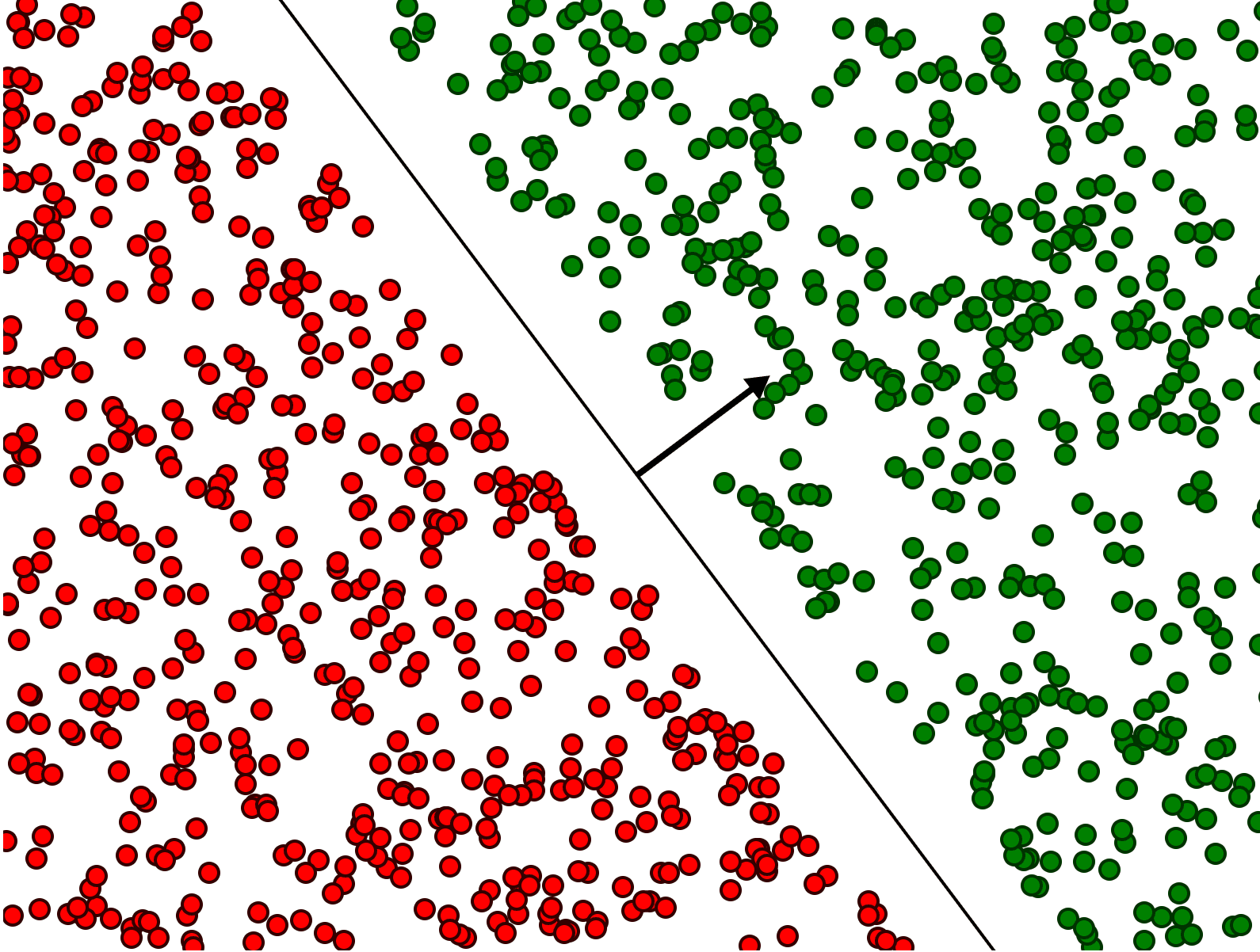
Let’s translate this to the parlance of machine-learning. Let $ x \in \mathbb{R}^n$ be a training data point, and $ y \in \{ 1, -1 \}$ is its label (green and red, in the images in this post). Suppose you want to find a hyperplane which separates all the points with -1 labels from those with +1 labels (assume for the moment that this is possible). For this and all examples in this post, we’ll use data in two dimensions, but the math will apply to any dimension.
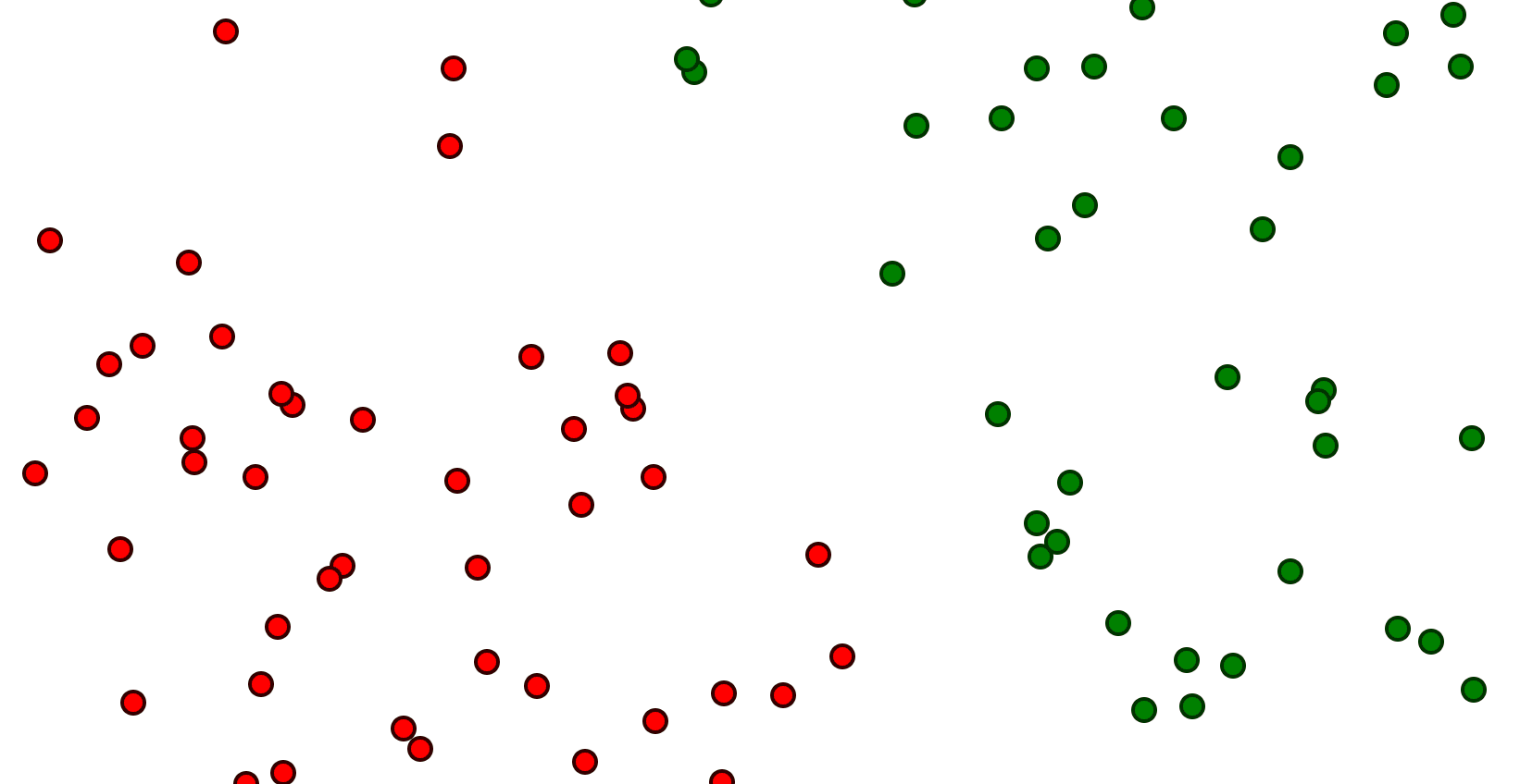
Some data labeled red and green, which is separable by a hyperplane (line).
The hypothesis we’re proposing to separate these points is a hyperplane, i.e. a linear subspace that splits all of $ \mathbb{R}^n$ into two halves. The data that represents this hyperplane is a single vector $ w$, the normal to the hyperplane, so that the hyperplane is defined by the solutions to the equation $ \langle x, w \rangle = 0$.
As we saw last time, $ w$ encodes the following rule for deciding if a new point $ z$ has a positive or negative label.
$$\displaystyle h_w(z) = \textup{sign}(\langle w, x \rangle)$$You’ll notice that this formula only works for the normals $ w$ of hyperplanes that pass through the origin, and generally we want to work with data that can be shifted elsewhere. We can resolve this by either adding a fixed term $ b \in \mathbb{R}$—often called a bias because statisticians came up with it—so that the shifted hyperplane is the set of solutions to $ \langle x, w \rangle + b = 0$. The shifted decision rule is:
$$\displaystyle h_w(z) = \textup{sign}(\langle w, x \rangle + b)$$Now the hypothesis is the pair of vector-and-scalar $ w, b$.
The key intuitive idea behind the formulation of the SVM problem is that there are many possible separating hyperplanes for a given set of labeled training data. For example, here is a gif showing infinitely many choices.
The question is: how can we find the separating hyperplane that not only separates the training data, but generalizes as well as possible to new data? The assumption of the SVM is that a hyperplane which separates the points, but is also as far away from any training point as possible, will generalize best.
While contrived, it’s easy to see that the separating hyperplane is as far as possible from any training point.
More specifically, fix a labeled dataset of points $ (x_i, y_i)$, or more precisely:
$$\displaystyle D = \{ (x_i, y_i) \mid i = 1, \dots, m, x_i \in \mathbb{R}^{n}, y_i \in \{1, -1\} \}$$And a hypothesis defined by the normal $ w \in \mathbb{R}^{n}$ and a shift $ b \in \mathbb{R}$. Let’s also suppose that $ (w,b)$ defines a hyperplane that correctly separates all the training data into the two labeled classes, and we just want to measure its quality. That measure of quality is the length of its margin.
Definition: The geometric margin of a hyperplane $ w$ with respect to a dataset $ D$ is the shortest distance from a training point $ x_i$ to the hyperplane defined by $ w$.
The best hyperplane has the largest possible margin.
This margin can even be computed quite easily using our work from last post. The distance from $ x$ to the hyperplane defined by $ w$ is the same as the length of the projection of $ x$ onto $ w$. And this is just computed by an inner product.
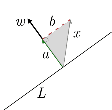
If the tip of the $ x$ arrow is the point in question, then $ a$ is the dot product, and $ b$ the distance from $ x$ to the hyperplane $ L$ defined by $ w$.
A naive optimization objective
If we wanted to, we could stop now and define an optimization problem that would be very hard to solve. It would look like this:
$$\displaystyle \begin{aligned} & \max_{w} \min_{x_i} \left | \left \langle x_i, \frac{w}{\|w\|} \right \rangle + b \right | & \\\ \textup{subject to \\ \\ } & \textup{sign}(\langle x_i, w \rangle + b) = \textup{sign}(y_i) & \textup{ for every } i = 1, \dots, m \end{aligned}$$The formulation is hard. The reason is it’s horrifyingly nonlinear. In more detail:
- The constraints are nonlinear due to the sign comparisons.
- There’s a min and a max! A priori, we have to do this because we don’t know which point is going to be the closest to the hyperplane.
- The objective is nonlinear in two ways: the absolute value and the projection requires you to take a norm and divide.
The rest of this post (and indeed, a lot of the work in grokking SVMs) is dedicated to converting this optimization problem to one in which the constraints are all linear inequalities and the objective is a single, quadratic polynomial we want to minimize or maximize.
Along the way, we’ll notice some neat features of the SVM.
Trick 1: linearizing the constraints
To solve the first problem, we can use a trick. We want to know whether $ \textup{sign}(\langle x_i, w \rangle + b) = \textup{sign}(y_i)$ for a labeled training point $ (x_i, y_i)$. The trick is to multiply them together. If their signs agree, then their product will be positive, otherwise it will be negative.
So each constraint becomes:
$$\displaystyle (\langle x_i, w \rangle + b) \cdot y_i \geq 0$$This is still linear because $ y_i$ is a constant (input) to the optimization problem. The variables are the coefficients of $ w$.
The left hand side of this inequality is often called the functional margin of a training point, since, as we will see, it still works to classify $ x_i$, even if $ w$ is scaled so that it is no longer a unit vector. Indeed, the sign of the inner product is independent of how $ w$ is scaled.
Trick 1.5: the optimal solution is midway between classes
This small trick is to notice that if $ w$ is the supposed optimal separating hyperplane, i.e. its margin is maximized, then it must necessarily be exactly halfway in between the closest points in the positive and negative classes.
In other words, if $ x_+$ and $ x_-$ are the closest points in the positive and negative classes, respectively, then $ \langle x_{+}, w \rangle + b = -(\langle x_{-}, w \rangle + b)$. If this were not the case, then you could adjust the bias, shifting the decision boundary along $ w$ until it they are exactly equal, and you will have increased the margin. The closest point, say $ x_+$ will have gotten farther away, and the closest point in the opposite class, $ x_-$ will have gotten closer, but will not be closer than $ x_+$.
Trick 2: getting rid of the max + min
Resolving this problem essentially uses the fact that the hypothesis, which comes in the form of the normal vector $ w$, has a degree of freedom in its length. To explain the details of this trick, we’ll set $ b=0$ which simplifies the intuition.
Indeed, in the animation below, I can increase or decrease the length of $ w$ without changing the decision boundary.
I have to keep my hand very steady (because I was too lazy to program it so that it only increases/decreases in length), but you can see the point. The line is perpendicular to the normal vector, and it doesn’t depend on the length.
Let’s combine this with tricks 1 and 1.5. If we increase the length of $ w$, that means the absolute values of the dot products $ \langle x_i, w \rangle $ used in the constraints will all increase by the same amount (without changing their sign). Indeed, for any vector $ a$ we have $ \langle a, w \rangle = \|w \| \cdot \langle a, w / \| w \| \rangle$.
In this world, the inner product measurement of distance from a point to the hyperplane is no longer faithful. The true distance is $ \langle a, w / \| w \| \rangle$, but the distance measured by $ \langle a, w \rangle$ is measured in units of $ 1 / \| w \|$.
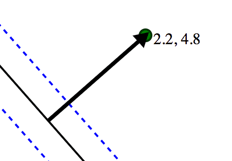
In this example, the two numbers next to the green dot represent the true distance of the point from the hyperplane, and the dot product of the point with the normal (respectively). The dashed lines are the solutions to <x, w> = 1. The magnitude of w is 2.2, the inverse of that is 0.46, and indeed 2.2 = 4.8 \* 0.46 (we’ve rounded the numbers).
Now suppose we had the optimal hyperplane and its normal $ w$. No matter how near (or far) the nearest positively labeled training point $ x$ is, we could scale the length of $ w$ to force $ \langle x, w \rangle = 1$. This is the core of the trick. One consequence is that the actual distance from $ x$ to the hyperplane is $ \frac{1}{\| w \|} = \langle x, w / \| w \| \rangle$.
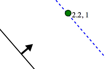
The same as above, but with the roles reversed. We’re forcing the inner product of the point with w to be 1. The true distance is unchanged.
In particular, if we force the closest point to have inner product 1, then all other points will have inner product at least 1. This has two consequences. First, our constraints change to $ \langle x_i, w \rangle \cdot y_i \geq 1$ instead of $ \geq 0$. Second, we no longer need to ask which point is closest to the candidate hyperplane! Because after all, we never cared which point it was, just how far away that closest point was. And now we know that it’s exactly $ 1 / \| w \|$ away. Indeed, if the optimal points weren’t at that distance, then that means the closest point doesn’t exactly meet the constraint, i.e. that $ \langle x, w \rangle > 1$ for every training point $ x$. We could then scale $ w$ shorter until $ \langle x, w \rangle = 1$, hence increasing the margin $ 1 / \| w \|$.
In other words, the coup de grâce, provided all the constraints are satisfied, the optimization objective is just to maximize $ 1 / \| w \|$, a.k.a. to minimize $ \| w \|$.
This intuition is clear from the following demonstration, which you can try for yourself. In it I have a bunch of positively and negatively labeled points, and the line in the center is the candidate hyperplane with normal $ w$ that you can drag around. Each training point has two numbers next to it. The first is the true distance from that point to the candidate hyperplane; the second is the inner product with $ w$. The two blue dashed lines are the solutions to $ \langle x, w \rangle = \pm 1$. To solve the SVM by hand, you have to ensure the second number is at least 1 for all green points, at most -1 for all red points, and then you have to make $ w$ as short as possible. As we’ve discussed, shrinking $ w$ moves the blue lines farther away from the separator, but in order to satisfy the constraints the blue lines can’t go further than any training point. Indeed, the optimum will have those blue lines touching a training point on each side.
svm_solve_by_hand
I bet you enjoyed watching me struggle to solve it. And while it’s probably not the optimal solution, the idea should be clear.
The final note is that, since we are now minimizing $ \| w \|$, a formula which includes a square root, we may as well minimize its square $ \| w \|^2 = \sum_j w_j^2$. We will also multiply the objective by $ 1/2$, because when we eventually analyze this problem we will take a derivative, and the square in the exponent and the $ 1/2$ will cancel.
The final form of the problem
Our optimization problem is now the following (including the bias again):
$$\displaystyle \begin{aligned} & \min_{w} \frac{1}{2} \| w \|^2 & \\\ \textup{subject to \\ \\ } & (\langle x_i, w \rangle + b) \cdot y_i \geq 1 & \textup{ for every } i = 1, \dots, m \end{aligned}$$This is much simpler to analyze. The constraints are all linear inequalities (which, because of linear programming, we know are tractable to optimize). The objective to minimize, however, is a convex quadratic function of the input variables—a sum of squares of the inputs.
Such problems are generally called quadratic programming problems (or QPs, for short). There are general methods to find solutions! However, they often suffer from numerical stability issues and have less-than-satisfactory runtime. Luckily, the form in which we’ve expressed the support vector machine problem is specific enough that we can analyze it directly, and find a way to solve it without appealing to general-purpose numerical solvers.
We will tackle this problem in a future post (planned for two posts sequel to this one). Before we close, let’s just make a few more observations about the solution to the optimization problem.
Support Vectors
In Trick 1.5 we saw that the optimal separating hyperplane has to be exactly halfway between the two closest points of opposite classes. Moreover, we noticed that, provided we’ve scaled $ \| w \|$ properly, these closest points (there may be multiple for positive and negative labels) have to be exactly “distance” 1 away from the separating hyperplane.
Another way to phrase this without putting “distance” in scare quotes is to say that, if $ w$ is the normal vector of the optimal separating hyperplane, the closest points lie on the two lines $ \langle x_i, w \rangle + b = \pm 1$.
Now that we have some intuition for the formulation of this problem, it isn’t a stretch to realize the following. While a dataset may include many points from either class on these two lines $ \langle x_i, w \rangle = \pm 1$, the optimal hyperplane itself does not depend on any of the other points except these closest points.
This fact is enough to give these closest points a special name: the support vectors.
We’ll actually prove that support vectors “are all you need” with full rigor and detail next time, when we cast the optimization problem in this post into the “dual” setting. To avoid vague names, the formulation described in this post called the “primal” problem. The dual problem is derived from the primal problem, with special variables and constraints chosen based on the primal variables and constraints. Next time we’ll describe in brief detail what the dual does and why it’s important, but we won’t have nearly enough time to give a full understanding of duality in optimization (such a treatment would fill a book).
When we compute the dual of the SVM problem, we will see explicitly that the hyperplane can be written as a linear combination of the support vectors. As such, once you’ve found the optimal hyperplane, you can compress the training set into just the support vectors, and reproducing the same optimal solution becomes much, much faster. You can also use the support vectors to augment the SVM to incorporate streaming data (throw out all non-support vectors after every retraining).
Eventually, when we get to implementing the SVM from scratch, we’ll see all this in action.
Until then!