Binary search is one of the most basic algorithms I know. Given a sorted list of comparable items and a target item being sought, binary search looks at the middle of the list, and compares it to the target. If the target is larger, we repeat on the smaller half of the list, and vice versa.
With each comparison the binary search algorithm cuts the search space in half. The result is a guarantee of no more than $ \log(n)$ comparisons, for a total runtime of $ O(\log n)$. Neat, efficient, useful.
There’s always another angle.
What if we tried to do binary search on a graph? Most graph search algorithms, like breadth- or depth-first search, take linear time, and they were invented by some pretty smart cookies. So if binary search on a graph is going to make any sense, it’ll have to use more information beyond what a normal search algorithm has access to.
For binary search on a list, it’s the fact that the list is sorted, and we can compare against the sought item to guide our search. But really, the key piece of information isn’t related to the comparability of the items. It’s that we can eliminate half of the search space at every step. The “compare against the target” step can be thought of a black box that replies to queries of the form, “Is this the thing I’m looking for?” with responses of the form, “Yes,” or, “No, but look over here instead.”

As long as the answers to your queries are sufficiently helpful, meaning they allow you to cut out large portions of your search space at each step, then you probably have a good algorithm on your hands. Indeed, there’s a natural model for graphs, defined in a 2015 paper of Emamjomeh-Zadeh, Kempe, and Singhal that goes as follows.
You’re given as input an undirected, weighted graph $ G = (V,E)$, with weights $ w_e$ for $ e \in E$. You can see the entire graph, and you may ask questions of the form, “Is vertex $ v$ the target?” Responses will be one of two things:
- Yes (you win!)
- No, but $ e = (v, w)$ is an edge out of $ v$ on a shortest path from $ v$ to the true target.
Your goal is to find the target vertex with the minimum number of queries.
Obviously this only works if $ G$ is connected, but slight variations of everything in this post work for disconnected graphs. (The same is not true in general for directed graphs)
When the graph is a line, this “reduces” to binary search in the sense that the same basic idea of binary search works: start in the middle of the graph, and the edge you get in response to a query will tell you in which half of the graph to continue.

And if we make this example only slightly more complicated, the generalization should become obvious:
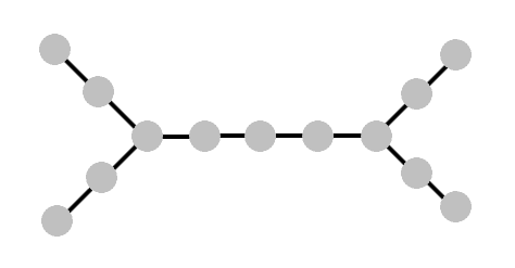
Here, we again start at the “center vertex,” and the response to our query will eliminate one of the two halves. But then how should we pick the next vertex, now that we no longer have a linear order to rely on? It should be clear, choose the “center vertex” of whichever half we end up in. This choice can be formalized into a rule that works even when there’s not such obvious symmetry, and it turns out to always be the right choice.
Definition: A median of a weighted graph $ G$ with respect to a subset of vertices $ S \subset V$ is a vertex $ v \in V$ (not necessarily in $ S$) which minimizes the sum of distances to vertices in $ S$. More formally, it minimizes
$ \Phi_S(v) = \sum_{u \in S} d(v, u)$,
where $ d(u,v)$ is the sum of the edge weights along a shortest path from $ v$ to $ u$.
And so generalizing binary search to this query-model on a graph results in the following algorithm, which whittles down the search space by querying the median at every step.
Algorithm: Binary search on graphs. Input is a graph $ G = (V,E)$.
- Start with a set of candidates $ S = V$.
- While we haven’t found the target and $ |S| > 1$:
- Query the median $ v$ of $ S$, and stop if you’ve found the target.
- Otherwise, let $ e = (v, w)$ be the response edge, and compute the set of all vertices $ x \in V$ for which $ e$ is on a shortest path from $ v$ to $ x$. Call this set $ T$.
- Replace $ S$ with $ S \cap T$.
- Output the only remaining vertex in $ S$
Indeed, as we’ll see momentarily, a python implementation is about as simple. The meat of the work is in computing the median and the set $ T$, both of which are slight variants of Dijkstra’s algorithm for computing shortest paths.
The theorem, which is straightforward and well written by Emamjomeh-Zadeh et al. (only about a half page on page 5), is that this algorithm requires only $ O(\log(n))$ queries, just like binary search.
Before we dive into an implementation, there’s a catch. Even though we are guaranteed only $ \log(n)$ many queries, because of our Dijkstra’s algorithm implementation, we’re definitely not going to get a logarithmic time algorithm. So in what situation would this be useful?
Here’s where we use the “theory” trick of making up a fanciful problem and only later finding applications for it (which, honestly, has been quite successful in computer science). In this scenario we’re treating the query mechanism as a black box. It’s natural to imagine that the queries are expensive, and a resource we want to optimize for. As an example the authors bring up in a followup paper, the graph might be the set of clusterings of a dataset, and the query involves a human looking at the data and responding that a cluster should be split, or that two clusters should be joined. Of course, for clustering the underlying graph is too large to process, so the median-finding algorithm needs to be implicit. But the essential point is clear: sometimes the query is the most expensive part of the algorithm.
Alright, now let’s implement it! The complete code is on Github as always.
Always be implementing
We start with a slight variation of Dijkstra’s algorithm. Here we’re given as input a single “starting” vertex, and we produce as output a list of all shortest paths from the start to all possible destination vertices.
We start with a bare-bones graph data structure.
from collections import defaultdict
from collections import namedtuple

Edge = namedtuple('Edge', ('source', 'target', 'weight'))

class Graph:
    # A bare-bones implementation of a weighted, undirected graph
    def __init__(self, vertices, edges=tuple()):
        self.vertices = vertices
        self.incident_edges = defaultdict(list)

        for edge in edges:
            self.add_edge(
                edge[0],
                edge[1],
                1 if len(edge) == 2 else edge[2]  # optional weight
            )

    def add_edge(self, u, v, weight=1):
        self.incident_edges[u].append(Edge(u, v, weight))
        self.incident_edges[v].append(Edge(v, u, weight))

    def edge(self, u, v):
        return [e for e in self.incident_edges[u] if e.target == v][0]
And then, since most of the work in Dijkstra’s algorithm is tracking information that you build up as you search the graph, we define the “output” data structure, a dictionary of edge weights paired with back-pointers for the discovered shortest paths.
class DijkstraOutput:
    def __init__(self, graph, start):
        self.start = start
        self.graph = graph

        # the smallest distance from the start to the destination v
        self.distance_from_start = {v: math.inf for v in graph.vertices}
        self.distance_from_start[start] = 0

        # a list of predecessor edges for each destination
        # to track a list of possibly many shortest paths
        self.predecessor_edges = {v: [] for v in graph.vertices}

    def found_shorter_path(self, vertex, edge, new_distance):
        # update the solution with a newly found shorter path
        self.distance_from_start[vertex] = new_distance

        if new_distance < self.distance_from_start[vertex]:
            self.predecessor_edges[vertex] = [edge]
        else:  # tie for multiple shortest paths
            self.predecessor_edges[vertex].append(edge)

    def path_to_destination_contains_edge(self, destination, edge):
        predecessors = self.predecessor_edges[destination]
        if edge in predecessors:
            return True
        return any(self.path_to_destination_contains_edge(e.source, edge)
                   for e in predecessors)

    def sum_of_distances(self, subset=None):
        subset = subset or self.graph.vertices
        return sum(self.distance_from_start[x] for x in subset)
The actual Dijkstra algorithm then just does a “breadth-first” (priority-queue-guided) search through $ G$, updating the metadata as it finds shorter paths.
def single_source_shortest_paths(graph, start):
    '''
    Compute the shortest paths and distances from the start vertex to all
    possible destination vertices. Return an instance of DijkstraOutput.
    '''
    output = DijkstraOutput(graph, start)
    visit_queue = [(0, start)]

    while len(visit_queue) > 0:
        priority, current = heapq.heappop(visit_queue)

        for incident_edge in graph.incident_edges[current]:
            v = incident_edge.target
            weight = incident_edge.weight
            distance_from_current = output.distance_from_start[current] + weight

            if distance_from_current <= output.distance_from_start[v]:
                output.found_shorter_path(v, incident_edge, distance_from_current)
                heapq.heappush(visit_queue, (distance_from_current, v))

    return output
Finally, we implement the median-finding and $ T$-computing subroutines:
def possible_targets(graph, start, edge):
    '''
    Given an undirected graph G = (V,E), an input vertex v in V, and an edge e
    incident to v, compute the set of vertices w such that e is on a shortest path from
    v to w.
    '''
    dijkstra_output = dijkstra.single_source_shortest_paths(graph, start)
    return set(v for v in graph.vertices
               if dijkstra_output.path_to_destination_contains_edge(v, edge))

def find_median(graph, vertices):
    '''
    Compute as output a vertex in the input graph which minimizes the sum of distances
    to the input set of vertices
    '''
    best_dijkstra_run = min(
         (single_source_shortest_paths(graph, v) for v in graph.vertices),
         key=lambda run: run.sum_of_distances(vertices)
    )
    return best_dijkstra_run.start
And then the core algorithm
QueryResult = namedtuple('QueryResult', ('found_target', 'feedback_edge'))

def binary_search(graph, query):
    '''
    Find a target node in a graph, with queries of the form "Is x the target?"
    and responses either "You found the target!" or "Here is an edge on a shortest
    path to the target."
    '''
    candidate_nodes = set(x for x in graph.vertices)  # copy

    while len(candidate_nodes) > 1:
        median = find_median(graph, candidate_nodes)
        query_result = query(median)

        if query_result.found_target:
            return median
        else:
            edge = query_result.feedback_edge
            legal_targets = possible_targets(graph, median, edge)
            candidate_nodes = candidate_nodes.intersection(legal_targets)

    return candidate_nodes.pop()
Here’s an example of running it on the example graph we used earlier in the post:
'''
Graph looks like this tree, with uniform weights

    a       k
     b     j
      cfghi
     d     l
    e       m
'''
G = Graph(['a', 'b', 'c', 'd', 'e', 'f', 'g', 'h', 'i',
           'j', 'k', 'l', 'm'],
          [
               ('a', 'b'),
               ('b', 'c'),
               ('c', 'd'),
               ('d', 'e'),
               ('c', 'f'),
               ('f', 'g'),
               ('g', 'h'),
               ('h', 'i'),
               ('i', 'j'),
               ('j', 'k'),
               ('i', 'l'),
               ('l', 'm'),
          ])

def simple_query(v):
    ans = input("is '%s' the target? [y/N] " % v)
    if ans and ans.lower()[0] == 'y':
        return QueryResult(True, None)
    else:
        print("Please input a vertex on the shortest path between"
              " '%s' and the target. The graph is: " % v)
        for w in G.incident_edges:
            print("%s: %s" % (w, G.incident_edges[w]))

        target = None
        while target not in G.vertices:
            target = input("Input neighboring vertex of '%s': " % v)

    return QueryResult(
        False,
        G.edge(v, target)
    )

output = binary_search(G, simple_query)
print("Found target: %s" % output)
The query function just prints out a reminder of the graph and asks the user to answer the query with a yes/no and a relevant edge if the answer is no.
An example run:
is 'g' the target? [y/N] n
Please input a vertex on the shortest path between 'g' and the target. The graph is:
e: [Edge(source='e', target='d', weight=1)]
i: [Edge(source='i', target='h', weight=1), Edge(source='i', target='j', weight=1), Edge(source='i', target='l', weight=1)]
g: [Edge(source='g', target='f', weight=1), Edge(source='g', target='h', weight=1)]
l: [Edge(source='l', target='i', weight=1), Edge(source='l', target='m', weight=1)]
k: [Edge(source='k', target='j', weight=1)]
j: [Edge(source='j', target='i', weight=1), Edge(source='j', target='k', weight=1)]
c: [Edge(source='c', target='b', weight=1), Edge(source='c', target='d', weight=1), Edge(source='c', target='f', weight=1)]
f: [Edge(source='f', target='c', weight=1), Edge(source='f', target='g', weight=1)]
m: [Edge(source='m', target='l', weight=1)]
d: [Edge(source='d', target='c', weight=1), Edge(source='d', target='e', weight=1)]
h: [Edge(source='h', target='g', weight=1), Edge(source='h', target='i', weight=1)]
b: [Edge(source='b', target='a', weight=1), Edge(source='b', target='c', weight=1)]
a: [Edge(source='a', target='b', weight=1)]
Input neighboring vertex of 'g': f
is 'c' the target? [y/N] n
Please input a vertex on the shortest path between 'c' and the target. The graph is:
[...]
Input neighboring vertex of 'c': d
is 'd' the target? [y/N] n
Please input a vertex on the shortest path between 'd' and the target. The graph is:
[...]
Input neighboring vertex of 'd': e
Found target: e
A likely story
The binary search we implemented in this post is pretty minimal. In fact, the more interesting part of the work of Emamjomeh-Zadeh et al. is the part where the response to the query can be wrong with some unknown probability.
In this case, there can be many shortest paths that are valid responses to a query, in addition to all the invalid responses. In particular, this rules out the strategy of asking the same query multiple times and taking the majority response. If the error rate is 1/3, and there are two shortest paths to the target, you can get into a situation in which you see three responses equally often and can’t choose which one is the liar.
Instead, the technique Emamjomeh-Zadeh et al. use is based on the Multiplicative Weights Update Algorithm (it strikes again!). Each query gives a multiplicative increase (or decrease) on the set of nodes that are consistent targets under the assumption that query response is correct. There are a few extra details and some postprocessing to avoid unlikely outcomes, but that’s the basic idea. Implementing it would be an excellent exercise for readers interested in diving deeper into a recent research paper (or to flex their math muscles).
But even deeper, this model of “query and get advice on how to improve” is a classic learning model first formally studied by Dana Angluin (my academic grand-advisor). In her model, one wants to design an algorithm to learn a classifier. The allowed queries are membership and equivalence queries. A membership is essentially, “What’s its label of this element?” and an equivalence query has the form, “Is this the right classifier?” If the answer is no, a mislabeled example is provided.
This is different from the usual machine learning assumption, because the learning algorithm gets to construct an example it wants to get more information about, instead of simply relying on a randomly generated subset of data. The goal is to minimize the number of queries before the target hypothesis is learned exactly. And indeed, as we saw in this post, if you have a little extra time to analyze the problem space, you can craft queries that extract quite a lot of information.
Indeed, the model we presented here for binary search on graphs is the natural analogue of an equivalence query for a search problem: instead of a mislabeled counterexample, you get a nudge in the right direction toward the target. Pretty neat!
There are a few directions we could take from here: (1) implement the Multiplicative Weights version of the algorithm, (2) apply this technique to a problem like ranking or clustering, or (3) cover theoretical learning models like membership and equivalence queries in more detail. What interests you?
Until next time!
Want to respond? Send me an email, post a webmention, or find me elsewhere on the internet.