Problem: Compute distance between points with uncertain locations (given by samples, or differing observations, or clusters).

For example, if I have the following three “points” in the plane, as indicated by their colors, which is closer, blue to green, or blue to red?

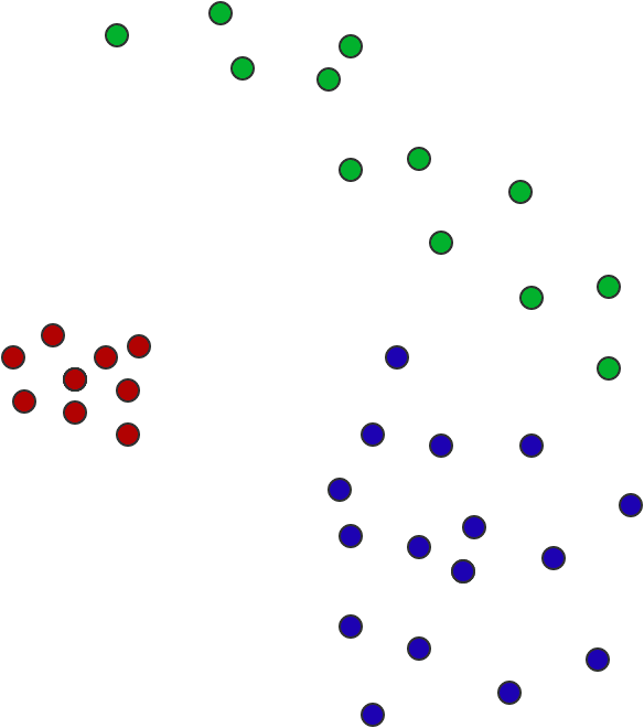
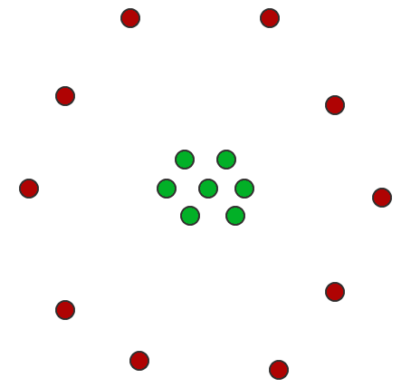
It’s not obvious, and there are multiple factors at work: the red points have fewer samples, but we can be more certain about the position; the blue points are less certain, but the closest non-blue point to a blue point is green; and the green points are equally plausibly “close to red” and “close to blue.” The centers of masses of the three sample sets are close to an equilateral triangle. In our example the “points” don’t overlap, but of course they could. And in particular, there should probably be a nonzero distance between two points whose sample sets have the same center of mass, as below. The distance quantifies the uncertainty.

All this is to say that it’s not obvious how to define a distance measure that is consistent with perceptual ideas of what geometry and distance should be.

Solution (Earthmover distance): Treat each sample set $ A$ corresponding to a “point” as a discrete probability distribution, so that each sample $ x \in A$ has probability mass $ p_x = 1 / |A|$. The distance between $ A$ and $ B$ is the optional solution to the following linear program.

Each $ x \in A$ corresponds to a pile of dirt of height $ p_x$, and each $ y \in B$ corresponds to a hole of depth $ p_y$. The cost of moving a unit of dirt from $ x$ to $ y$ is the Euclidean distance $ d(x, y)$ between the points (or whatever hipster metric you want to use).

Let $ z_{x, y}$ be a real variable corresponding to an amount of dirt to move from $ x \in A$ to $ y \in B$, with cost $ d(x, y)$. Then the constraints are:

• Each $ z_{x, y} \geq 0$, so dirt only moves from $ x$ to $ y$.
• Every pile $ x \in A$ must vanish, i.e. for each fixed $ x \in A$, $ \sum_{y \in B} z_{x,y} = p_x$.
• Likewise, every hole $ y \in B$ must be completely filled, i.e. $ \sum_{y \in B} z_{x,y} = p_y$.

The objective is to minimize the cost of doing this: $ \sum_{x, y \in A \times B} d(x, y) z_{x, y}$.

In python, using the ortools library (and leaving out a few docstrings and standard import statements, full code on Github):

from ortools.linear_solver import pywraplp

def earthmover_distance(p1, p2):
    dist1 = {x: count / len(p1) for (x, count) in Counter(p1).items()}
    dist2 = {x: count / len(p2) for (x, count) in Counter(p2).items()}
    solver = pywraplp.Solver('earthmover_distance', pywraplp.Solver.GLOP_LINEAR_PROGRAMMING)

    variables = dict()

    # for each pile in dist1, the constraint that says all the dirt must leave this pile
    dirt_leaving_constraints = defaultdict(lambda: 0)

    # for each hole in dist2, the constraint that says this hole must be filled
    dirt_filling_constraints = defaultdict(lambda: 0)

    # the objective
    objective = solver.Objective()
    objective.SetMinimization()

    for (x, dirt_at_x) in dist1.items():
        for (y, capacity_of_y) in dist2.items():
            amount_to_move_x_y = solver.NumVar(0, solver.infinity(), 'z_{%s, %s}' % (x, y))
            variables[(x, y)] = amount_to_move_x_y
            dirt_leaving_constraints[x] += amount_to_move_x_y
            dirt_filling_constraints[y] += amount_to_move_x_y
            objective.SetCoefficient(amount_to_move_x_y, euclidean_distance(x, y))

    for x, linear_combination in dirt_leaving_constraints.items():
        solver.Add(linear_combination == dist1[x])

    for y, linear_combination in dirt_filling_constraints.items():
        solver.Add(linear_combination == dist2[y])

    status = solver.Solve()
    if status not in [solver.OPTIMAL, solver.FEASIBLE]:
        raise Exception('Unable to find feasible solution')

    return objective.Value()

Discussion: I’ve heard about this metric many times as a way to compare probability distributions. For example, it shows up in an influential paper about fairness in machine learning, and a few other CS theory papers related to distribution testing.

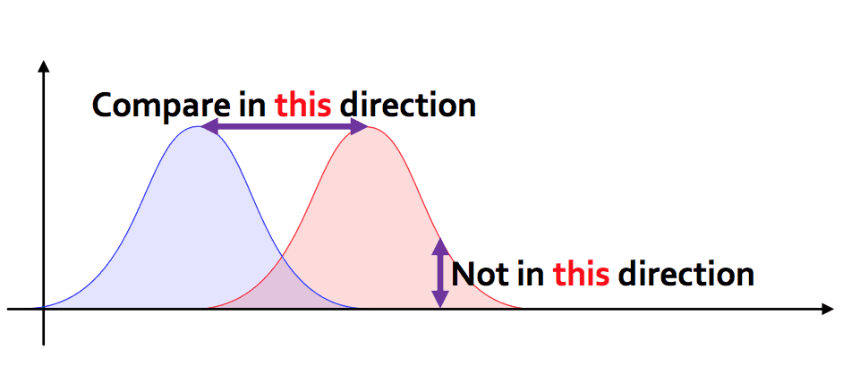
One might ask: why not use other measures of dissimilarity for probability distributions (Chi-squared statistic, Kullback-Leibler divergence, etc.)? One answer is that these other measures only give useful information for pairs of distributions with the same support. An example from a talk of Justin Solomon succinctly clarifies what Earthmover distance achieves

Also, why not just model the samples using, say, a normal distribution, and then compute the distance based on the parameters of the distributions? That is possible, and in fact makes for a potentially more efficient technique, but you lose some information by doing this. Ignoring that your data might not be approximately normal (it might have some curvature), with Earthmover distance, you get point-by-point details about how each data point affects the outcome.

This kind of attention to detail can be very important in certain situations. One that I’ve been paying close attention to recently is the problem of studying gerrymandering from a mathematical perspective. Justin Solomon of MIT is a champion of the Earthmover distance (see his fascinating talk here for more, with slides) which is just one topic in a field called “optimal transport.”

This has the potential to be useful in redistricting because of the nature of the redistricting problem. As I wrote previously, discussions of redistricting are chock-full of geometry—or at least geometric-sounding language—and people are very concerned with the apparent “compactness” of a districting plan. But the underlying data used to perform redistricting isn’t very accurate. The people who build the maps don’t have precise data on voting habits, or even locations where people live. Census tracts might not be perfectly aligned, and data can just plain have errors and uncertainty in other respects. So the data that district-map-drawers care about is uncertain much like our point clouds. With a theory of geometry that accounts for uncertainty (and the Earthmover distance is the “distance” part of that), one can come up with more robust, better tools for redistricting.

Solomon’s website has a ton of resources about this, under the names of “optimal transport” and “Wasserstein metric,” and his work extends from computing distances to computing important geometric values like the barycenter, computational advantages like parallelism.

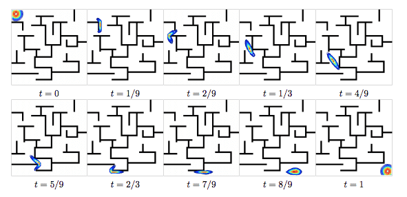
Others in the field have come up with transparency techniques to make it clearer how the Earthmover distance relates to the geometry of the underlying space. This one is particularly fun because the explanations result in a path traveled from the start to the finish, and by setting up the underlying metric in just such a way, you can watch the distribution navigate a maze to get to its target. I like to imagine tiny ants carrying all that dirt.

Finally, work of Shirdhonkar and Jacobs provide approximation algorithms that allow linear-time computation, instead of the worst-case-cubic runtime of a linear solver.